Nested if for 12 results? Can it be done?

Churchy LaFemme

Board Regular
Joined
Sep 22, 2010
Messages
135
This nested if in a shared workbook is getting unwieldly. The one thing I can do, what I hope to do, is update the IF statement in Column I, Status, so that if always works.

The status text strings are found in the cells above columns 0 though P. (That is, the if refences are to O2, P2, etc.) Data inputs are always dates.

There are two basic flows – Monkey is from the US, or not from the US.
If from the US, we skip two steps.

There are two variables.
1. A non-US monkey may have quarantine set right away, set during reviews process, or it may already have happened and the “Monkey in Quarantine status will never appear. (One of the current problems is that if someone inputs the date that quarantine was set, the row will immediately show a later stage status, making it appear we have completed more steps than we have.

2. Assessments may be resubmitted.
– Either the director returns an assessment with questions, and we resubmit after addressing questions - Or we may realize we need to update and then resubmit resubmit (We’ve had problems where once something has been returned or resubmitted, that status sticks in “Director Reviewing”

First step is that once we have a date in Column, the first status should be triggered for that row. That is, one we input a date in column O, a status appears in column I. Column U may also be completed at the point, which is where this started falling apart. (The table is actually A-AL, but only columns that are part of this beastly IF are shown.)

Ignore the top row and the left-hand column. Those are not part of the table in my worksheet. Uploads are disabled (work) so I had to paste from Excel.

Complete IntakeDirector Reviewing AssessmentAddress QuestionsDirector Reviewing AssessmentVet Finalizing AssessmentMonkey in QuarantineMonkey Introduced to GroupMonkey AcclimatingDirector DeterminationDetermination
Column AColumn IColumn OColumn PColumn QColumn RColumn SColumn TColumn UColumn VColumn QColumn X
COUNTRYSTATUSMonkey ArrivedAssessment SubmittedDirector Returns w QuestionsResubmit AssessmentDirector ApproveVet Sets QuarantineMonkey Completes QuarantineStaff Manages & MonitorsDetermination - Sanctuary or RehomeMonkey Set for Stay or Rehome
USComplete IntakeDATAIGNORE - may or may not have data
Case 1Director Reviewing AssessmentDATA
Case 2Director Reviewing AssessmentDATADATA
Address QuestionsDATADATAIGNORE - may or may not have data
Vet Finalizing AssessmentDATAIGNORE - may or may not have data
Monkey in QuarantineDATABLANK
Case 1Monkey Introduced to GroupDATADATA
Case 2Skip if Column A is "US"IGNORE if Column A is "US"
Case 1Monkey AcclimatingDATA
Case 2Skip if Column A is "US"IGNORE if Column A is "US"
Director DeterminationDATA
DeterminationDATA

If there is a good tutorial somewhere that explains how to structure Nested IF statements to this level of complexity, that would be helpful.

I'm hoping someone has already build such a creature, and can provide the blueprint.
 

Excel Facts

Which came first: VisiCalc or Lotus 1-2-3?
Dan Bricklin and Bob Frankston debuted VisiCalc in 1979 as a Visible Calculator. Lotus 1-2-3 debuted in the early 1980's, from Mitch Kapor.
Would you be able to provide exact details of how the process works?

Which cell is filled in first and with what kind of data? Which cells react to this data being entered and what are the conditions on how they react?

Which cell is next to be filled in? Etc..

And what formula(s) you are already using.
 
Upvote 0
Column O is always first, we may or may not input a date for column U at that point.
So then that status tells us to build up the assessment and log the date in column P. From here the ideal we next log and date in column S, but we may end up using Columns Q and R. (I though about just deleted the date submission date if returned or resubmitted, but then it looks like it was never submitted for the person who is only tracking the space between intake and assessment.)
If and only if S has a date, we move on.
If column A is not US, then we can skip steps.

Reordering columns is not an option as I not the owner of the workbook and there are many columns with other stuff.
This should be the formula. =IF([@[Monkey Set for Stay or Rehome]]="",IF([@[Determination - Sanctuary or Rehome]]="",IF([@[Staff Manages & Monitors]]="",IF([@[Monkey Completes Quarantine]]="",IF([@[Vet Sets Quarantine]]="",IF([@[Director Approve]]="",IF([@[Resubmit Assessment]]="",IF([@[Director Returns w Questions]]="",IF([@[Assessment Submitted]]="",IF(AND([@[Monkey Arrived]]="",I7=""),"",O$4),P$4),Q$4),R$4),S$4),T$4),IF([@Country]="US",W$4,U$4)),V$4),W$4),X$4)

My best guess is that the formula is wonky because they added new triggers as they were needed - not so much in order of when things happen. But I don't know for sure.

(I'm working in a downloaded copy with a limited data set the formula is what we have in the shared file.)
 
Upvote 0
Ok, so that doesn't really explain how the process works. I mean, I understand that you fill in a date in one cell, and another should produce a result based on that date, but.. you didn't explain it step by step. Pretend I am a new hire with absolutely no experience with this worksheet and you're teaching me how to use it from the very beginning.

And what data is in row 4?
 
Upvote 0
Ah, I see the issue. It is really painful to do this without a living spreadsheet.
For the purposes of the text-table, "row 4" is the first line of the table. Row 3 is the header row, and row 2 is not part of the table.

The first input would be the date of an arrival. Column O. This will trigger the status column to show that you should "complete intake."
The rest of my lengthy reply was eaten! I will try again shortly.
NOTE: Notice that when I was trying to format column letters and name to BOLD, I turned W in to Q.
 
Upvote 0
Okay, new hire.
O The first input would be the date of an arrival. Column O. This will trigger the status column to show that you should "complete intake." We may or may not have a date for column U which should not effect the status (yet).
P Next step is to submit the assessment. Log the date in column P, and the status should be "director reviewing assessment."

Q & R Most often, the assessment comes back (with or without changes) and you do not need to use columns Q or R.
If the assessment is returned with questions, log the date in column Q and the status should be "Address Questions" ....
until you resubmit and log the date in column R, which puts the status back at "director reviewing assessment."

S When the director has returned the final, log the date in column S which triggers the status "Vet Finalizing Assessment" (This happens automatically when the director is done - you don't have any interactions here. )

T When the vet has finalized, we finally care about column U. Log the date for the Vet Sets Quarantine.

U Most likely, there is not already a date in column U. If column U is blank when you input the date in column T, then the status should be "Monkey In Quarantine." If there was already date, the status is "Monkey Introduced to Group" unless column A is US. If the row has US in column A, the status is "Director Determination." (The Q end date will be sent - you don't know in advance. Despite the name of Column T.)

V Only used if column A is not "US". The column name is a little misleading, but basically there is another assessment and when you get it, you log the date in column V and the the status goes to "Director Determination."

W When the determinate comes back, log that date and the status changes to "Determination" and we are done!

Does that make sense? At all?
 
Upvote 0
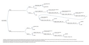
I find when building IF statements PowerPoint or something similar works well for thinking through and visualizing the logic.

Flow.jpg
 
Upvote 1
Okay, new hire.
O The first input would be the date of an arrival. Column O. This will trigger the status column to show that you should "complete intake." We may or may not have a date for column U which should not effect the status (yet).
P Next step is to submit the assessment. Log the date in column P, and the status should be "director reviewing assessment."

Q & R Most often, the assessment comes back (with or without changes) and you do not need to use columns Q or R.
If the assessment is returned with questions, log the date in column Q and the status should be "Address Questions" ....
until you resubmit and log the date in column R, which puts the status back at "director reviewing assessment."

S When the director has returned the final, log the date in column S which triggers the status "Vet Finalizing Assessment" (This happens automatically when the director is done - you don't have any interactions here. )

T When the vet has finalized, we finally care about column U. Log the date for the Vet Sets Quarantine.

U Most likely, there is not already a date in column U. If column U is blank when you input the date in column T, then the status should be "Monkey In Quarantine." If there was already date, the status is "Monkey Introduced to Group" unless column A is US. If the row has US in column A, the status is "Director Determination." (The Q end date will be sent - you don't know in advance. Despite the name of Column T.)

V Only used if column A is not "US". The column name is a little misleading, but basically there is another assessment and when you get it, you log the date in column V and the the status goes to "Director Determination."

W When the determinate comes back, log that date and the status changes to "Determination" and we are done!

Does that make sense? At all?
Yes, I believe that made sense. See if this does what you want:

Excel Formula:
=IF(AND(O4<>"",COUNTA(P4:T4)<1,COUNTA(V4:W4)<1),"Complete Intake",IF(OR(AND(P4<>"",COUNTA(Q4:T4)<1,COUNTA(V4:W4)<1),AND(R4<>"",COUNTA(S4:T4)<1,COUNTA(V4:W4)<1)),"Director Reviewing Assessment",IF(AND(Q4<>"",COUNTA(R4:T4)<1,COUNTA(V4:W4)<1),"Address Questions",IF(AND(S4<>"",T4="",COUNTA(V4:W4)<1),"Vet Finalizing Assessment",IF(AND(T4<>"",U4="",COUNTA(V4:W4)<1),"Monkey In Quarantine",IF(AND(T4<>"",U4<>"",COUNTA(V4:W4)<1,A4<>"US"),"Monkey Introduced To Group",IF(OR(AND(T4<>"",U4<>"",W4="",A4="US"),AND(A4<>"US",V4<>"",W4="")),"Director Determination",IF(W4<>"","Determination",""))))))))
 
Upvote 1
Another option. Not sure if this is what you want when "US" in column A:

Book1
AHIOPQRSTUVWX
1Complete IntakeDirector Reviewing AssessmentAddress QuestionsDirector Reviewing AssessmentVet Finalizing AssessmentMonkey in QuarantineMonkey Introduced to GroupMonkey AcclimatingDirector DeterminationDetermination
2Column AExpected resultColumn IColumn OColumn PColumn QColumn RColumn SColumn TColumn UColumn VColumn QColumn X
3COUNTRYSTATUSMonkey ArrivedAssessment SubmittedDirector Returns w QuestionsResubmit AssessmentDirector ApproveVet Sets QuarantineMonkey Completes QuarantineStaff Manages & MonitorsDetermination - Sanctuary or RehomeMonkey Set for Stay or Rehome
4 
5Complete IntakeComplete IntakeDATA
6Director Reviewing AssessmentDirector Reviewing AssessmentDATADATA
7Address QuestionsAddress QuestionsDATADATADATA
8Director Reviewing AssessmentDirector Reviewing AssessmentDATADATADATADATA
9Vet Finalizing AssessmentVet Finalizing AssessmentDATADATADATADATADATA
10Monkey in QuarantineMonkey in QuarantineDATADATADATADATADATADATA
11Monkey Introduced to GroupMonkey Introduced to GroupDATADATADATADATADATADATADATA
12Monkey AcclimatingMonkey AcclimatingDATADATADATADATADATADATADATADATA
13Director DeterminationDirector DeterminationDATADATADATADATADATADATADATADATADATA
14DeterminationDeterminationDATADATADATADATADATADATADATADATADATADATA
15USComplete IntakeComplete IntakeDATA
16USDirector Reviewing AssessmentDirector Reviewing AssessmentDATADATA
17USAddress QuestionsAddress QuestionsDATADATADATA
18USDirector Reviewing AssessmentDirector Reviewing AssessmentDATADATADATADATA
19USVet Finalizing AssessmentVet Finalizing AssessmentDATADATADATADATADATA
20USMonkey in QuarantineMonkey in QuarantineDATADATADATADATADATADATA
21USMonkey Introduced to GroupDirector DeterminationDATADATADATADATADATADATADATA
22USMonkey AcclimatingDirector DeterminationDATADATADATADATADATADATADATADATA
23USDirector DeterminationDirector DeterminationDATADATADATADATADATADATADATADATADATA
24USDeterminationDeterminationDATADATADATADATADATADATADATADATADATADATA
Sheet1
Cell Formulas
RangeFormula
I4:I24I4=LET(statuses,{"Complete Intake","Director Reviewing Assessment","Address Questions","Director Reviewing Assessment","Vet Finalizing Assessment","Monkey in Quarantine","Monkey Introduced to Group","Monkey Acclimating","Director Determination","Determination"}, p,MAX(SEQUENCE(,10)*(O4:X4<>"")), r,IF(p>0,INDEX(statuses,,p),""), test,IF(A4="US",SUBSTITUTE(SUBSTITUTE(r,"Monkey Introduced to Group","Director Determination"),"Monkey Acclimating","Director Determination"),r), test )
 
Last edited:
Upvote 0

Forum statistics

Threads
1,215,069
Messages
6,122,959
Members
449,096
Latest member
Anshu121

We've detected that you are using an adblocker.

We have a great community of people providing Excel help here, but the hosting costs are enormous. You can help keep this site running by allowing ads on MrExcel.com.
Allow Ads at MrExcel

Which adblocker are you using?

Disable AdBlock

Follow these easy steps to disable AdBlock

1)Click on the icon in the browser’s toolbar.
2)Click on the icon in the browser’s toolbar.
2)Click on the "Pause on this site" option.
Go back

Disable AdBlock Plus

Follow these easy steps to disable AdBlock Plus

1)Click on the icon in the browser’s toolbar.
2)Click on the toggle to disable it for "mrexcel.com".
Go back

Disable uBlock Origin

Follow these easy steps to disable uBlock Origin

1)Click on the icon in the browser’s toolbar.
2)Click on the "Power" button.
3)Click on the "Refresh" button.
Go back

Disable uBlock

Follow these easy steps to disable uBlock

1)Click on the icon in the browser’s toolbar.
2)Click on the "Power" button.
3)Click on the "Refresh" button.
Go back
Back
Top