One cell input - multiple conditions and outputs.

[Mikey556]

Good afternoon valued excel experts, I respectuflly request your help!

I am creating a spreadsheet for work. We have many employees who have an insane number of courses that must be completed throughout the year, all with varying expiry lengths (in days). I have tried to simplify with a basic mock spreadsheet to explain what we want to achieve (attached).

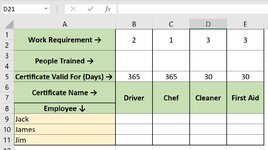
Situation: I input a date for 'Driver' course completion, for Jack in cell B9.

What I require from the spreadsheet from this one input:

1. The B9 cell will immediately turn green, if in date (after checking certificate validity length in days from B5).
2. The B9 cell will turn red, once it expires the 365 day limit, as dictated by B5.
3. The B3 cell will check all dates in the 'driver' column (B9:B11) and show how many are in date (true?).
4. The B3 cell will turn green/red, if the 'work requirement' (B1) is met/not met. (eg. we require 2 drivers at all times, all 3 employees are in date for driving certificate = cell turns green).

I hope I didn't make this too long winded. Any help would be HUGELY appreciated and I'll be eternally grateful.

Thankfully,

Mikey.

Book1
	A	B	C	D	E
1	Work Requirement →	2	1	3	3
2
3	People Trained →
4
5	Certificate Valid For (Days) →	365	365	30	30
6	Certificate Name →	Driver	Chef	Cleaner	First Aid
7
8	Employee ↓
9	Jack
10	James
11	Jim
Sheet1

 

[gordsky]

I think this can be done with some conditional formatting and a countif. You can of course need to manipulate the ranges to suit and copy across but the below will work for your driver column....

create a conditional format for each of the below formula (if you're unsure how to google has good examples). Make sure the "$" are exactly as below

 =AND($B9<>"",TODAY()>$B9+$B$5) .... applies to =$B$3 ....format/fill to red
 =AND($B9<>"",TODAY()<$B9+$B$5) .... applies to =$B$3 ....format/fill to green
 =AND($B9<>"",TODAY()>$B9+$B$5).... applies to =$B$9:$B$11....format/fill to red
 =AND($B9<>"",TODAY()<$B9+$B$5).... applies to =$B$9:$B$11....format/fill to green

In cell B3 enter the following formula

=COUNTIF(B9:B11,">" & TODAY()-B5)

 

[Mikey556]

I think this can be done with some conditional formatting and a countif. You can of course need to manipulate the ranges to suit and copy across but the below will work for your driver column....

create a conditional format for each of the below formula (if you're unsure how to google has good examples). Make sure the "$" are exactly as below

 =AND($B9<>"",TODAY()>$B9+$B$5) .... applies to =$B$3 ....format/fill to red
 =AND($B9<>"",TODAY()<$B9+$B$5) .... applies to =$B$3 ....format/fill to green
 =AND($B9<>"",TODAY()>$B9+$B$5).... applies to =$B$9:$B$11....format/fill to red
 =AND($B9<>"",TODAY()<$B9+$B$5).... applies to =$B$9:$B$11....format/fill to green

In cell B3 enter the following formula

=COUNTIF(B9:B11,">" & TODAY()-B5)

gordsky,

I cannot thank you enough! I managed the first few issues through hours of googling and work arounds, but came unstuck at the end. That COUNTIF line has really saved the day!

Consider this case closed and thanks again, you absolute Excel Wizard ?‍!