Payment terms (formula) for P&L impact and Cash flow

[Adfinance]

Hi everyone, how are you?
Could I ask you to help me please?

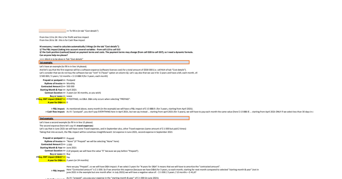
I need to calculate automatically 2 things (see the link below - in the tab "Cost details"):
1/ The P&L impact (taking into account several variables - from cell L13 to cell S13
2/ the Cash position (cashout) based on payment terms, total cost expense, start month and date, etc.. The payment terms may change (from cell D28 to cell D37), so I need dynamic formulas.
Can anyone help me please?

All the details to help you are displayed in the Excel file, in the tab "Instructions". And your outcome will be in the tab "Cost details".
Thank you soooo much for your help, it would be really helpful to me.

Link to access the excel file here:

To send to Mr Excel - version 1.xlsx

docs.google.com

@maabadi

 

[maabadi]

I think Worksheet Change Event very Good for you (Post #59), Only you need input data and then macro run automatically.
if you still want excel normal complex formula, I could work on it, but maybe it take very long time & it will be impossible.

 

[maabadi]

If you want Complex Formula. This is it. But Before Do it. I add one sheet to your file and some source for finding K & Vlookup Value within Formula. Then I also Upload your file with added worksheet. You can Hide that sheet if want.
This is Formula at AJ14:

=IF($L14="Prepaid",IF($R14="BUY",IF($S14="YES",IF(COLUMN()=FormulaAssumptions!$F14,$N14*-1,IF($T14=0,"",IF(AND(COLUMN()>FormulaAssumptions!$F14,COLUMN()<FormulaAssumptions!$F14+12*$T14+1,MOD(COLUMN()-FormulaAssumptions!$F14-1,VLOOKUP($M14,Table1,3,FALSE))=0),$N14*-1/(VLOOKUP($M14,Table1,2,FALSE)*$T14),""))),IF(COLUMN()=FormulaAssumptions!$F14,$N14*-1,"")),IF($S14="NO",IF($Q14=0,"",IF(AND(COLUMN()>FormulaAssumptions!$F14-1,COLUMN()<FormulaAssumptions!$F14+12*$Q14,MOD(COLUMN()-FormulaAssumptions!$F14,VLOOKUP($M14,Table1,3,FALSE))=0),$N14*-1/(VLOOKUP($M14,Table1,2,FALSE)*$Q14),"")),IF(COLUMN()=FormulaAssumptions!$F14,$N14*-1,""))),IF($R14="BUY",IF(COLUMN()=FormulaAssumptions!$F14,$N14*-1,""),IF($S14="YES",IF($T14=0,"",IF(AND(COLUMN()>FormulaAssumptions!$F14+VLOOKUP($M14,Table1,3,FALSE)-1,COLUMN()<FormulaAssumptions!$F14+VLOOKUP($M14,Table1,3,FALSE)+12*$T14+1,MOD(COLUMN()-FormulaAssumptions!$F14-VLOOKUP($M14,Table1,3,FALSE)-1,VLOOKUP($M14,Table1,3,FALSE))=0),$N14*-1/(VLOOKUP($M14,Table1,2,FALSE)*$T14),"")),IF($S14="NO",IF(AND(COLUMN()>FormulaAssumptions!$F14-1,COLUMN()<FormulaAssumptions!$F14+12*$Q14,MOD(COLUMN()-FormulaAssumptions!$F14,VLOOKUP($M14,Table1,3,FALSE))=0),$N14*-1/(VLOOKUP($M14,Table1,2,FALSE)*$Q14),""),
IF(COLUMN()=FormulaAssumptions!$F14,$N14*-1,"")))))

At this file I added All codes also ( if you don't want them Delete Codes. See Post #60 to know how delete No. 1).
1. Worksheet Change Event Code
2. UDF (User Defined Function)
3. Normal Formula
4. Normal Macro.

This formula Version is Slow & Take Time to open and respond. For me, Worksheet Change Event is Best.
Model for Maabadi (30.05.21) vF - Macro Enabled

 

[Adfinance]

About above formula if you see very zero values and don't want them Try this at AJ28 then Drag it:

=IF(COLUMNS($AJ:AJ) - 1 >= $D28,IF(ISBLANK(OFFSET(AJ14,0, $D28*-1,1,1)),"",OFFSET(AJ14,0, $D28*-1,1,1)),"")

What is Problem with VBA Code?
1. if you have problem with need to run after inputting data. you can use Worksheet change event Macro. this macro automatically run after input data as specific Cells. only you need save file as Macro-Enabled Workbook(.xlsm)
For this, at excel Window, Right click on sheet Cost Details & Select View Code, then Paste this code and save file as Macro-Enabled Workbook(.xlsm)

Private Sub Worksheet_Change(ByVal Target As Range)
Dim i As Long, j As Long, K As Long, Lr As Long, Lc As Long, Sh As Worksheet
Dim M As Double, L As Long, N As Long, P As Long, x As Long, arr(1 To 5, 1 To 2)
Set Sh = Sheets("Cost Details")
With Sh
If Intersect(Target, Union(.Range("L14:T23"), .Range("L44:T53"), .Range("L74:T83"))) Is Nothing Then Exit Sub
i = Target.Row
P = Application.WorksheetFunction.CountA(.Range("L" & i & ":T" & i))
If P < 9 Then Exit Sub
Application.EnableEvents = False
Lc = .Cells(13, Columns.Count).End(xlToLeft).Column
x = 1
Range(.Cells(i, 36), .Cells(i, Lc)).ClearContents
    arr(1, 1) = "Annually": arr(2, 1) = "Bi-annually": arr(3, 1) = "Quarterly"
    arr(4, 1) = "Monthly": arr(5, 1) = "Non applicable": arr(1, 2) = 1
    arr(2, 2) = 2: arr(3, 2) = 4: arr(4, 2) = 12: arr(5, 2) = 12
        N = 12 / arr(Application.Match(Range("M" & i).Value, Application.Index(arr, 0, 1), 0), 2)
        K = Application.WorksheetFunction.EoMonth(.Range("O" & i).Value, .Range("P" & i).Value) - 1
        K = Application.WorksheetFunction.Match(K, Range(.Cells(13, 1), .Cells(13, Lc)))
    If .Range("L" & i).Value = "Prepaid" Then
        If .Range("R" & i).Value = "BUY" Then
            If .Range("S" & i).Value = "YES" Then
                .Cells(i, K).Value = .Range("N" & i).Value * -1
                 If .Range("T" & i).Value = 0 Then
                       GoTo Step2
                 Else
                 L = (12 / N) * .Range("T" & i).Value
                 M = (.Range("N" & i).Value / L) * -1
                  For j = K + N To K + N - 1 + 12 * .Range("T" & i).Value Step N
                   .Cells(i, j).Value = M
                  Next j
                 End If
            ElseIf .Range("S" & i).Value = "NO" Then
              .Cells(i, K).Value = .Range("N" & i).Value * -1
            End If

        ElseIf .Range("R" & i).Value = "LEASE" Then
            If .Range("S" & i).Value = "NO" Then
              If .Range("Q" & i).Value = 0 Then
                    GoTo Step2
              Else
                L = (12 / N) * .Range("Q" & i).Value
                M = (.Range("N" & i).Value / L) * -1
                For j = K To K - 1 + 12 * .Range("Q" & i).Value Step N
                  .Cells(i, j).Value = M
                Next j
              End If
            ElseIf .Range("S" & i).Value = "YES" Then
                .Cells(i, K).Value = .Range("N" & i).Value * -1
            End If
        End If

    End If

    If .Range("L" & i).Value = "Postpaid" Then
        If .Range("R" & i).Value = "BUY" Then
           .Cells(i, K).Value = .Range("N" & i).Value * -1
            If .Range("S" & i).Value = "YES" Then

                 If .Range("T" & i).Value = 0 Then
                       GoTo Step2
                 Else
                    L = (12 / N) * .Range("T" & i).Value
                    M = (.Range("N" & i).Value / L) * -1

                For j = K + N To K + N - 1 + 12 * .Range("T" & i).Value Step N
                  .Cells(i, j).Value = M
                Next j
                End If
            End If
        ElseIf .Range("R" & i).Value = "LEASE" Then
            If .Range("S" & i).Value = "NO" Then
                    L = (12 / N) * .Range("Q" & i).Value
                    M = (.Range("N" & i).Value / L) * -1
                For j = K To K - 1 + 12 * .Range("Q" & i).Value Step N
                  .Cells(i, j).Value = M
                Next j
            ElseIf .Range("S" & i).Value = "YES" Then
                .Cells(i, K).Value = .Range("N" & i).Value * -1
            End If
        End If
    End If
Step2:
End With
Application.EnableEvents = True
End Sub

2. for formula, it maybe possible & if possible, it would be very long & Complex formula.

Hi @maabadi

1/ About the formula for Payment terms : Perfect! Thank you. Great work!
2/ About the VBA code, actually it works very well (for now). The only problem is that we will change and modify and file in the future. And the VBA code will be impacted. And maybe it won't work anymore, if columns have changed, etc.
This is the reason why I think that a dynamic formula would be THE BEST. In the sense that, even if we change something in our file or our tab "cost details", there won't be any problem with it thanks to the formula.

Do you think you can send me a formula, that fulfils the same job as the VBA code?

3/ About UDF code, still confusing. I don't know how to manage it.

Thank you so much for your help!

 

[maabadi]

I Sent Formula at Post #62. Only you need to have sheet I added at your workbook ( Sheet FormulaAssumptions).

 

[Adfinance]

I Sent Formula at Post #62. Only you need to have sheet I added at your workbook ( Sheet FormulaAssumptions).

Thank you for the formula. The "drag and drop" does not work for the entire values (only talking about the formula).

For some cells, there is the following error " #NAME?". Could you help me with this issue please?
@maabadi

 

[maabadi]

Download file I shared at Post #62 & with instruction I told at that post, test it.

 

[Adfinance]

@maabadi thank you!

 

[Adfinance]

@maabadi thank you!

@maabadi

Would it be possible to modify this please?

1/ Tab "Cost details"
In the cash flow impact (from line 28 to 37, from line 58 to 67, from line 88 to 97) we only want the values from column N to be displayed here : " Total contracted amount $".

I explain myself ... if BUY we will have an EBIT impact. In the "Cash flow impact", we only want the value(s) from the "total contracted amount" ... NOTHING ABOUT THE VALUES FROM EBIT IMPACT.
Is it possible?

Thank you so much!
@maabadi

 

[maabadi]

Please tell with example.

 

[Adfinance]

Please tell with example.

Hi @maabadi ... To be more specific ...
When you have an expense (cost), you will have (today or in the future) a cash disbursement. This is the reason why I divided the tab "Cost details" into 2 parts (i) P&L impact (for expenses) and (ii) Cash flow impact (for cash disbursements).

Here, the thing I want you to solve is the following.

In column "N" (tab "cost details") we have the "total contracted amount" in $ ... this is the EXPENSE.
So ... in your formula (and VBA code ... if it is about the "total contracted amount" ... let it be in "Cash impact" table (from line 28 to 37, from line 58 to 67, from line 88 to 97).

If it's about EBIT impact ... then every value from EBIT impact has to be taken out from the Cash flow impact tables ....


Some examples:

1/ "BUY" .. so "EBIT impact" is "YES" :
Here when selecting "BUY", only the first value on the left (for each line I mean) in the P&L impact tables will be displayed in Cash flow tables
For instance, in line 14 we selected BUY, with a "total contracted amount" of - 1 000 000 $ (and a "start month and year" which is 22/06/21).
So in the P&L impact table >>> - 1 000 000 $ in 06/21 (ad other value yes, but for EBIT impact ... we only take the value from "total contracted amount" in the below table of Cash flow impact .... related with payment terms).
So ... finally here, this total value will be displayed in 06/21 in the Cash flow table (in the example, line 28, cell AJ28) if we select +0 month at cell D28.

The same rules apply for every line, when we select "BUY" .... we only take (for the cash flow impact tables) the value(s) from the "total contracted amount" .... NOT from the EBIT impact.

2/ "LEASE" .. so "EBIT impact" is "NO" :
Here when selecting LEASE, all the value from the P&L impact will also be displayed in the Cash flow impact (the only difference will be the payment terms (+0 month, +1 month, +2 months, etc.). So, when "LEASE" selected, NOTHING TO CHANGE/MODIFY here.

think the proper way would be to say (for Cash flow impact - post #68) :
> If "BUY" selection, put only the first value on the left (to be displayed in the cash flow impact section) because the first value represents the "total contracted amount" ... and the other are not relevant because they are part of EBIT impact.
> If "LEASE" selection, let's put every value (to be displayed in the cash flow section) because the sum of everything here represents the "total contracted amount" and NOT the EBIT impact ... because NO EBIT impact in the LEASE option).