Private Sub Worksheet_Change(ByVal Target As Range)
Dim i As Long, J As Long, Lr1 As Long, Lr2 As Long, Cr1 As Long, Cr1R As String, Cr2 As Long, Cr2R As String
Dim Lr3 As Long, Lr4 As Long, M1 As Long, M2 As Long, Cr3 As Variant, M As Long
On Error Resume Next
Lr1 = Range("I" & Rows.Count).End(xlUp).Row + Target.Rows.Count - 1
Lr2 = Range("N" & Rows.Count).End(xlUp).Row + Target.Rows.Count - 1
If Intersect(Target, Union(Range("I3:I" & Lr1), Range("N3:N" & Lr2))) Is Nothing Then Exit Sub
Lr3 = Sheets("Work").Range("A" & Rows.Count - 20).End(xlUp).Row
Lr4 = Sheets("Paper").Range("A" & Rows.Count - 20).End(xlUp).Row
Application.FindFormat.Clear
Application.EnableEvents = False
If Not Intersect(Target, Range("I3:I" & Lr1)) Is Nothing Then
M = Application.WorksheetFunction.Match(Range("I" & Target.Row - 1), Sheets("Work").Range("A1:A" & Lr3), 0)
If M = 0 Then
M1 = 1
Else
Application.FindFormat.Interior.Color = 4697456
M1 = Sheets("Work").Range("A" & M + 2 & ":A" & Lr3).Find("", , , , , xlNext, , , True).Row
End If
M2 = Application.WorksheetFunction.Match(Range("I" & Target.Row), Sheets("Work").Range("A1:A" & Lr3), 0) - 1
Application.FindFormat.Interior.Color = 14277081
If M2 = 0 Then M2 = Sheets("Work").Range("A" & M1 + 2 & ":A" & Lr3 + 100).Find("", , , , , xlNext, , , True).Row
Sheets("Work").Rows(M1 & ":" & M2).Delete
Sheets("Work").Rows(Lr3 + 100).Resize(M2 - M1 + 1).Insert
Range("J3:J" & Lr1 - Target.Rows.Count + 1).Formula = "=IFERROR(INDEX(Work!B:B,MATCH($I4,Work!A:A,0)-2,0),"""")"
Range("K3:K" & Lr1 - Target.Rows.Count + 1).Formula = "=IFERROR(SUM(INDEX(Work!D:D,MATCH($I3,Work!A:A,0)+1,0):INDEX(Work!E:E,MATCH($I4,Work!A:A,0)-2,0)),"""")"
Range("L3:L" & Lr1 - Target.Rows.Count + 1).Formula = "=IFERROR(SUM(INDEX(Work!F:F,MATCH($I3,Work!A:A,0)+1,0):INDEX(Work!G:G,MATCH($I4,Work!A:A,0)-2,0)),"""")"
For i = Target.Row To Lr1 - Target.Rows.Count + 1
If i = Lr1 - Target.Rows.Count + 1 Then GoTo Resum4
Cr1 = Application.WorksheetFunction.Match(Range("I" & i), Sheets("Work").Range("A1:A" & Lr3), 0)
Cr1R = Range("A" & Cr1).Address
Range("I" & i).Hyperlinks.Delete
Sheets("Dashboard").Hyperlinks.Add Anchor:=Range("I" & i), Address:="", SubAddress:="'" & Sheets("Work").Name & "'!" & Cr1R, TextToDisplay:=Range("I" & i).Value
With Sheets("Dashboard").Range("I" & i)
.Font.Underline = xlUnderlineStyleNone
.Font.ColorIndex = xlColorIndexAutomatic
.Font.Name = "Microsoft Parsi"
.Font.Size = 14
.HorizontalAlignment = xlCenter
.VerticalAlignment = xlCenter
End With
Next i
Resum4:
M2 = Application.WorksheetFunction.Match("New Customer", Sheets("Dashboard").Range("I1:I" & Lr1), 0)
Sheets("Dashboard").Range("J" & M2 & ":L" & M2 + Target.Rows.Count - 1).Delete Shift:=xlUp
End If
If Not Intersect(Target, Range("N3:N" & Lr2)) Is Nothing Then
M = Application.WorksheetFunction.Match(Range("N" & Target.Row - 1), Sheets("Paper").Range("A1:A" & Lr4), 0)
If M = 0 Then
M1 = 1
Else
Application.FindFormat.Interior.Color = 12874308
M1 = Sheets("Paper").Range("A" & M + 2 & ":A" & Lr4).Find("", , , , , xlNext, , , True).Row
End If
M2 = Application.WorksheetFunction.Match(Range("N" & Target.Row), Sheets("Paper").Range("A1:A" & Lr4), 0) - 1
Application.FindFormat.Interior.Color = 14277081
If M2 = 0 Then M2 = Sheets("Paper").Range("A" & M1 + 2 & ":A" & Lr4 + 100).Find("", , , , , xlNext, , , True).Row
Sheets("Paper").Rows(M1 & ":" & M2).Delete
Sheets("Paper").Rows(Lr4 + 100).Resize(M2 - M1 + 1).Insert
Range("O3:O" & Lr2 - Target.Rows.Count + 1).Formula = "=IFERROR(INDEX(Paper!B:B,MATCH($N4,Paper!A:A,0)-2,0),"""")"
Range("P3:P" & Lr2 - Target.Rows.Count + 1).Formula = "=IFERROR(SUM(INDEX(Paper!D:D,MATCH($N3,Paper!A:A,0)+1,0):INDEX(Paper!E:E,MATCH($N4,Paper!A:A,0)-2,0)),"""")"
Range("Q3:Q" & Lr2 - Target.Rows.Count + 1).Formula = "=IFERROR(SUM(INDEX(Paper!F:F,MATCH($N3,Paper!A:A,0)+1,0):INDEX(Paper!G:G,MATCH($N4,Paper!A:A,0)-2,0)),"""")"
For i = Target.Row To Lr2 - Target.Rows.Count + 1
If i = Lr2 - Target.Rows.Count + 1 Then GoTo Resum5
Cr1 = Application.WorksheetFunction.Match(Range("N" & i), Sheets("Paper").Range("A1:A" & Lr4), 0)
Cr1R = Range("A" & Cr1).Address
Range("N" & i).Hyperlinks.Delete
Sheets("Dashboard").Hyperlinks.Add Anchor:=Range("N" & i), Address:="", SubAddress:="'" & Sheets("Paper").Name & "'!" & Cr1R, TextToDisplay:=Range("N" & i).Value
With Sheets("Dashboard").Range("N" & i)
.Font.Underline = xlUnderlineStyleNone
.Font.ColorIndex = xlColorIndexAutomatic
.Font.Name = "Microsoft Parsi"
.Font.Size = 14
.HorizontalAlignment = xlCenter
.VerticalAlignment = xlCenter
End With
Next i
Resum5:
M2 = Application.WorksheetFunction.Match("New Customer", Sheets("Dashboard").Range("N1:N" & Lr2), 0)
Sheets("Dashboard").Range("O" & M2 & ":Q" & M2 + Target.Rows.Count - 1).Delete Shift:=xlUp
End If
Application.FindFormat.Clear
Application.EnableEvents = True
End Sub
Private Sub Worksheet_SelectionChange(ByVal Target As Range)
Dim i As Long, J As Long, Lr1 As Long, Lr2 As Long, Cr1 As Long, Cr1R As String, Cr2 As Long, Cr2R As String
Dim Lr3 As Long, Lr4 As Long, M1 As Long, M2 As Long, Cr3 As Variant
Lr1 = Range("I" & Rows.Count).End(xlUp).Row
Lr2 = Range("N" & Rows.Count).End(xlUp).Row
Lr3 = Sheets("Work").Range("A" & Rows.Count - 20).End(xlUp).Row
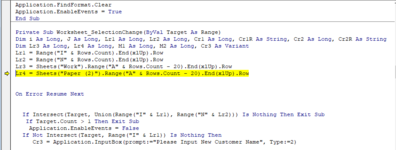
Lr4 = Sheets("Paper (2)").Range("A" & Rows.Count - 20).End(xlUp).Row
On Error Resume Next
If Intersect(Target, Union(Range("I" & Lr1), Range("N" & Lr2))) Is Nothing Then Exit Sub
If Target.Count > 1 Then Exit Sub
Application.EnableEvents = False
If Not Intersect(Target, Range("I" & Lr1)) Is Nothing Then
Cr3 = Application.InputBox(prompt:="Please Input New Customer Name", Type:=2)
If Cr3 = False Then
Application.EnableEvents = True
Exit Sub
Else
Range("I" & Lr1 & ":M" & Lr1).Insert Shift:=xlDown
i = Application.WorksheetFunction.Match(Cr3, Sheets("Work").Range("A1:A" & Lr3), 0)
If i = False Then
Application.FindFormat.Clear
Application.FindFormat.Interior.Color = 4697456
i = Sheets("Work").Range("A" & Lr3 + 3 & ":A" & Rows.Count).Find("", , , , , xlNext, , , True).Row
Sheets("Dashboard").Range("I" & Lr1).Value = Cr3
Worksheets("Dashboard").Sort.SortFields.Clear
Range("I2:I" & Lr1).Sort Key1:=Range("I2"), Header:=xlYes, Order1:=xlAscending
M2 = Application.WorksheetFunction.Match(Cr3, Sheets("Dashboard").Range("I1:I" & Lr1), 0)
M1 = Application.WorksheetFunction.Match(Sheets("Dashboard").Range("I" & M2 + 1).Value, Sheets("Work").Range("A1:A" & Lr3), 0)
Application.FindFormat.Interior.Color = 14277081
If M1 = 0 Then M1 = Sheets("Work").Range("A1:A" & Lr3 + 100).Find("", , , , , xlNext, , , True).Row + 1
If M1 = 0 Then M1 = 1
Sheets("Work").Range("A" & i & ":G" & i + 3).Copy
Sheets("Work").Range("A" & M1 & ":G" & M1).Insert Shift:=xlDown
Sheets("Work").Range("A" & M1).Value = Cr3
Sheets("Work").Range("A" & M1).Font.ColorIndex = xlColorIndexAutomatic
Sheets("Work").Rows(i).Resize(4).Delete
End If
End If
Range("J3:J" & Lr1).Formula = "=IFERROR(INDEX(Work!B:B,MATCH($I4,Work!A:A,0)-2,0),"""")"
Range("K3:K" & Lr1).Formula = "=IFERROR(SUM(INDEX(Work!D:D,MATCH($I3,Work!A:A,0)+1,0):INDEX(Work!E:E,MATCH($I4,Work!A:A,0)-2,0)),"""")"
Range("L3:L" & Lr1).Formula = "=IFERROR(SUM(INDEX(Work!F:F,MATCH($I3,Work!A:A,0)+1,0):INDEX(Work!G:G,MATCH($I4,Work!A:A,0)-2,0)),"""")"
For i = M2 To Lr1
Cr1 = Application.WorksheetFunction.Match(Range("I" & i), Sheets("Work").Range("A1:A" & Lr3), 0)
Cr1R = Range("A" & Cr1).Address
Range("I" & i).Hyperlinks.Delete
Sheets("Dashboard").Hyperlinks.Add Anchor:=Range("I" & i), Address:="", SubAddress:="'" & Sheets("Work").Name & "'!" & Cr1R, TextToDisplay:=Range("I" & i).Value
With Sheets("Dashboard").Range("I" & i)
.Font.Underline = xlUnderlineStyleNone
.Font.ColorIndex = xlColorIndexAutomatic
.Font.Name = "Microsoft Parsi"
.Font.Size = 14
.HorizontalAlignment = xlCenter
.VerticalAlignment = xlCenter
End With
Next i
Sheets("Work").Activate
Sheets("Work").Range("A" & M1).Select
Application.EnableEvents = True
End If
If Not Intersect(Target, Range("N" & Lr2)) Is Nothing Then
If Target.Count = 1 Then
Application.EnableEvents = False
Cr3 = Application.InputBox(prompt:="Please Input New Customer Name", Type:=2)
If Cr3 = False Then
Application.EnableEvents = True
Exit Sub
Else
Range("N" & Lr2 & ":Q" & Lr2).Insert Shift:=xlDown
i = Application.WorksheetFunction.Match(Cr3, Sheets("Paper").Range("A1:A" & Lr4), 0)
If i = False Then
Application.FindFormat.Clear
Application.FindFormat.Interior.Color = 4697456
i = Sheets("Paper").Range("A" & Lr4 + 3 & ":A" & Rows.Count).Find("", , , , , xlNext, , , True).Row
Sheets("Dashboard").Range("N" & Lr2).Value = Cr3
Worksheets("Dashboard").Sort.SortFields.Clear
Range("N2:N" & Lr2).Sort Key1:=Range("N2"), Header:=xlYes, Order1:=xlAscending
M2 = Application.WorksheetFunction.Match(Cr3, Sheets("Dashboard").Range("N1:N" & Lr2), 0)
M1 = Application.WorksheetFunction.Match(Sheets("Dashboard").Range("N" & M2 + 1).Value, Sheets("Paper").Range("A1:A" & Lr4), 0)
Application.FindFormat.Interior.Color = 14277081
If M1 = 0 Then M1 = Sheets("Paper").Range("A1:A" & Lr4 + 100).Find("", , , , , xlNext, , , True).Row + 1
If M1 = 0 Then M1 = 1
Sheets("Paper").Range("A" & i & ":G" & i + 3).Copy
Sheets("Paper").Range("A" & M1 & ":G" & M1).Insert Shift:=xlDown
Sheets("Paper").Range("A" & M1).Value = Cr3
Sheets("Paper").Range("A" & M1).Font.ColorIndex = xlColorIndexAutomatic
End If
End If
Range("O3:O" & Lr2).Formula = "=IFERROR(INDEX(Paper!B:B,MATCH($N4,Paper!A:A,0)-2,0),"""")"
Range("P3:P" & Lr2).Formula = "=IFERROR(SUM(INDEX(Paper!D:D,MATCH($N3,Paper!A:A,0)+1,0):INDEX(Paper!E:E,MATCH($N4,Paper!A:A,0)-2,0)),"""")"
Range("Q3:Q" & Lr2).Formula = "=IFERROR(SUM(INDEX(Paper!F:F,MATCH($N3,Paper!A:A,0)+1,0):INDEX(Paper!G:G,MATCH($N4,Paper!A:A,0)-2,0)),"""")"
For i = M2 To Lr2
Cr1 = Application.WorksheetFunction.Match(Range("N" & i), Sheets("Paper").Range("A1:A" & Lr4), 0)
Cr1R = Range("A" & Cr1).Address
Range("N" & i).Hyperlinks.Delete
Sheets("Dashboard").Hyperlinks.Add Anchor:=Range("N" & i), Address:="", SubAddress:="'" & Sheets("Paper").Name & "'!" & Cr1R, TextToDisplay:=Range("N" & i).Value
With Sheets("Dashboard").Range("N" & i)
.Font.Underline = xlUnderlineStyleNone
.Font.ColorIndex = xlColorIndexAutomatic
.Font.Name = "Microsoft Parsi"
.Font.Size = 14
.HorizontalAlignment = xlCenter
.VerticalAlignment = xlCenter
End With
Next i
Sheets("Paper").Activate
Sheets("Paper").Range("A" & M1).Select
End If
End If
Application.FindFormat.Clear
Application.EnableEvents = True
End Sub
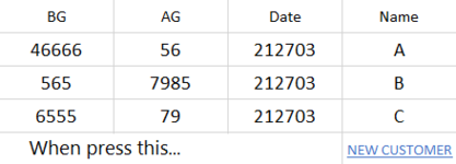
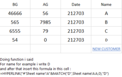
") however like ever you right and i wrong, but how about 1? this is main problem that make mistakes when i working on last customer that i be careful not write on this 4 source rows sample of insert new customers
however like ever you right and i wrong, but how about 1? this is main problem that make mistakes when i working on last customer that i be careful not write on this 4 source rows sample of insert new customers