Removing the need of a helper column

Marvo

Board Regular
Joined
Nov 27, 2023
Messages
155
Office Version
  1. 2021
Platform
  1. Windows
Good morning, yesterday I posed a question regarding the attached image and Stephen Crump kindly gave me the perfect solution.

=COUNTIFS(A2:A34,"League",B2:B34,"H",D2:D34,E14)

What has got me thinking is the solution doesn't reference column C at all and as column D is a helper column that refers to Column C, is it possible to "cut out the middle man" completely, meaning I could dispense with the helper column? It would be a great boon if so as the several helper columns (60 in all) really slow the workbook down.

The formula in D3 is =IF(($A3="League")*($B3="H"),IF($C3="W",SUM(1,D2),0),N(D2))

Copied down

Many thanks for any help offered and if it can't be done, so be it. Just wondered.
 

Attachments

  • Mr Excel.JPG
    Mr Excel.JPG
    79.2 KB · Views: 29
I've been working all day trying to figures out how to sort Alphabetically if you name are John Smith for example. First came a points total, then alphabetical. I scoured the internet high and low, watched some you utube and couldn't find a solution, one expert said it couldn't be done (red flag to a bull that is) without a separate column for both the first name and surname.
Well I did it, opened a new worksheet, listed all the players alphabetically, gave them an ID Number (1 = Brian Adams, 250 = Zac Zebedee) then used VBA, to sort by the points total, then by the ID number and bingo. Full name in one cell, spelt the wrong way (so to speak) then ID number. I was really chuffed. Good thing was, if you added a player or took one away, it still works.
 
Upvote 0

Excel Facts

Did you know Excel offers Filter by Selection?
Add the AutoFilter icon to the Quick Access Toolbar. Select a cell containing Apple, click AutoFilter, and you will get all rows with Apple
Hi. I've been looking at this all day and I've come to the conclusion its just beyond me. I literally have no idea where to start. What I have now since I removed the helper columns is a workbook two thirds of the size that is working quite quickly so I think it best if I left things as they were. Somebody could do this for me but what would be the point, if something went wrong I'd have no idea how to put it right.

Maybe I'll try and make some smaller adjustments, a little bit at a time.

I apologise for all the work you've put in, I've no doubt it's brilliant but I'm completely lost. Sorry.
 
Upvote 0
*Since I removed the formula in the helper columns.
 
Upvote 0
No apologies needed!...I understand your perspective. The formula is focused on the main challenge of eliminating the long helper columns that involve sequential row-by-row calculations. It does that and more, but whether that's necessary now is debatable. Since you've hardwired the results of those helper calculations, and workbook performance is now acceptable, the approach I've mapped out may very well be a solution in search of a different problem. In order to make the formula easier to maintain (difficult to say with a straight face), I've attempted to generalize it so that the same formula can be applied without modification to the first three subsections of the summary table (for W, L, and D). To do that, of course, the formula needs some inputs that were previously hardwired into different variations of your original formula. These inputs need to be set up in some local helper cells (the orange cells in my earlier example) around the summary table. Once that is done, assuming the source data column mappings are correct, you should get results that (hopefully) make sense. I have an idea for making modest extensions to the formula so that it would also work on the Goals Scored and Goals Conceded subsections.

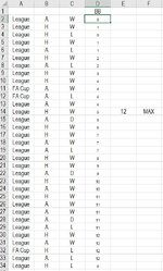
But a lot happens inside the formula that will require some study time to see how the formula works. Are you familiar with how to view an intermediate result inside a LET function? If not, I would recommend setting up a small example---one that can be readily examined by eye to confirm that intermediate results make sense. The example below would be a good starting point. I've slightly altered the layout from the example in post #28 to show dates in two formats (because internal to the formula, all dates are numerical, not in dd/mm/yyyy format), so this extra numerical date column facilitates comparisons with results from the formula. And the four input cells are shifted so that the "outcome" appears in the same column as the formula, and the other three inputs appear on a row to the left (although not all three on the same row to keep the example from sprawling across the screen too far). You should be able to copy the example directly from this post (using the small clipboard icon in the upper left of the minisheet), and paste it into cell B1 of an empty worksheet (the same cell shown in the upper left of the posted minisheet). That should duplicate what is shown, other than setting up data validation lists for the four input (blue) cells...or you can simply type the desired query inputs in those cells. The single formula has been edited slightly, by giving the final output formula a variable name, and then after the final formula, we can type the name of any variable that should be displayed by the formula. I've called the formula that generates the final results, the three-cell spilling array, "finres"...so the last variable in the formula would be finres to see the final result. But if you want to see the "rary" array or the filtered data "fd" array, simply replace the last formula argument with the appropriate variable name. The example below shows the revised filtered array "revfd" that I described earlier. It offers a clear visualization of the streaks present. I recommend using the detailed description in post #28 and step through each of the variables in the formula to visualize the operations. Then try different inputs and alter the data table to create various types of streaks to confirm the performance.

Feel free to post back with any questions, suggestions, or reports of incorrect results.
MrExcel_20240321 (version 1).xlsx
BEJKLMNOPQRSTU
1outcomes -->W
2DateLocationMatch TypeResultGoals ScoredGoals ConcededNumerical DateTOTALTIMES DATES
301/02/2024ALeagueW3245323match locationAll45323W
402/02/2024HLeagueL1245324match typeAll||
503/02/2024HLeagueL0245325calc typewoOpp||
604/02/2024HFA CupD334532645326D
705/02/2024ALeagueL1345327||
806/02/2024HLeagueW424532845328W
907/02/2024ALeagueW134532945329W
1008/02/2024HLeagueW014533045330W
1109/02/2024HLeagueL1345331||
1210/02/2024HFA CupW524533245332W
1311/02/2024AFA CupL2345333||
1412/02/2024ALeagueW324533445334W
1513/02/2024HLeagueW224533545335W
1614/02/2024ALeagueD114533645336D
1715/02/2024HLeagueW414533745337W
18
Sheet5
Cell Formulas
RangeFormula
S3:T17S3=LET(loc, Q3, mt, Q4, ct, Q5, oc, S1, src, $B3:$M10000, fsrc, FILTER(src, INDEX(src, , 10) <> ""), data, INDEX(fsrc, SEQUENCE(ROWS(fsrc)), {1,4,9,10}), opp, XLOOKUP(oc, {"W","L","D"}, {"L","W","D"}), allr_data, SEQUENCE(ROWS(data), , 1, 0), loc_ary, IF(loc = "All", allr_data, INDEX(data, , 2) = loc), mt_ary, IF(mt = "All", allr_data, INDEX(data, , 3) = mt), fd, FILTER(INDEX(data, SEQUENCE(ROWS(data)), {1,4}), loc_ary * mt_ary), allr_fd, SEQUENCE(ROWS(fd)), revfd, IF(SWITCH(ct, "wOnly", INDEX(fd, , 2) = oc, "woOpp", INDEX(fd, , 2) <> opp), INDEX(fd, allr_fd, {1,2}), {"|","|"}), rstr, CONCAT(INDEX(revfd, , 2)), rary, IFERROR(FILTERXML("<x><y>" & SUBSTITUTE(rstr, "|", "</y><y>") & "</y></x>", "//y"), ""), ls, LEN(rary), maxs, MAX(ls), nmaxs, SUM(--(ls = maxs)), csum_ls, MMULT(--(SEQUENCE(1, ROWS(ls)) <= SEQUENCE(ROWS(ls))), ls), idxs_ls, FILTER(SEQUENCE(ROWS(ls)), ls = maxs), idxs_dts, INDEX(csum_ls, idxs_ls), seds, INDEX(FILTER(INDEX(revfd, , 1), INDEX(revfd, , 1) <> "|"), idxs_dts), dt_comp, TEXTJOIN(", ", , IFERROR(TEXT(INDEX(seds, SEQUENCE(nmaxs - 1)), "yyyy"), ""), TEXT(INDEX(seds, nmaxs), "dd/mm/yyyy")), finres, IF(maxs = 0, {"none","",""}, CHOOSE({1,2,3}, maxs, nmaxs, dt_comp)), revfd )
N3:N17N3=B3
Dynamic array formulas.
Cells with Data Validation
CellAllowCriteria
S1ListW,L,D
Q3ListH,A,All
Q4ListLeague,All
Q5ListwOnly,woOpp
 
Upvote 0
The thing that came to my mind was, in the boxes, I don't need then to say VICTORIES, DRAWS OR DEFEATS, or GOALS SCORED or CONCEDED, could be just W, D, L, GF & GA. HOME or AWAY could be just H & A. Something like this would be much easier for me to follow.
Cobblers.xlsm
ABCDEFGHIJKLMNOPQ
1ALL-TIME RECORDS
2CONSECUTIVESW D LGFGA
3TOTALTIMESSTART/END DATETOTALTIMESSTART/END DATETOTALTIMESSTART/END DATETOTALTIMESSTART/END DATETOTALTIMESSTART/END DATE
4ALLALL11128/12/1899621983 & 2011741972, 1985, 1988 & 199228103/10/190829128/12/1965
5MatchesH14116/04/19275121/03/1981621985 & 200254128/01/092816113/10/1900
6A622004 & 2015421913 & 199416127/10/190619127/03/195940101/09/1926
7lgeALL11128/12/1899621983 & 20118126/10/193528129/08/201527128/09/1965
8MatchesH1221899 & 20275121/03/1981551905, 1985, 1999, 2002 & 201675128/12/192619113/10/1900
9A8121/11/20155106/09/199415127/10/190618127/03/195942120/02/1965
10LONGEST RUNSNO LNO DNO WNO GANO GF
11TOTALTIMESSTART/END DATETOTALTIMESSTART/END DATETOTALTIMESSTART/END DATETOTALTIMESSTART/END DATETOTALTIMESSTART/END DATE
12ALLALL27123/01/201629105/02/19271921969 & 1993621910 & 19307107/04/1939
13MatchesH33122/02/191328131/08/195711117/01/19909125/08/19236114/12/2002
14A14113/02/201621112/04/190828127/01/19066112/04/1997721938 & 1995
15lgeALL31128/12/201529105/02/19271821969 & 2011621930 & 19757107/04/1939
16MatchesH33122/02/19132621898 & 198411117/01/19909125/08/19235114/12/2002
17A19131/10/201523130/04/196633101/01/19216112/04/19978128/03/1967
Records
Cell Formulas
RangeFormula
C4C4=LET(t,ALL!$K:$K,s,SEQUENCE(ROWS(t)),MAX(FREQUENCY(IF(t="W",s),IF(t<>"W",s))))
C5C5=LET(t,FILTER(ALL!$K:$K,ALL!$E:$E="H"),MAX(FREQUENCY(IF(t="W",SEQUENCE(ROWS(t))),IF(t<>"W",SEQUENCE(ROWS(t))))))
C6C6=LET(t,FILTER(ALL!$K:$K,ALL!$E:$E="A"),MAX(FREQUENCY(IF(t="W",SEQUENCE(ROWS(t))),IF(t<>"W",SEQUENCE(ROWS(t))))))
C7C7=LET(t,FILTER(ALL!$K:$K,ALL!$J:$J="League"),MAX(FREQUENCY(IF(t="W",SEQUENCE(ROWS(t))),IF(t<>"W",SEQUENCE(ROWS(t))))))
C8C8=LET(t,FILTER(ALL!$K:$K,(ALL!$J:$J="League")*(ALL!$E:$E="H")),s,SEQUENCE(ROWS(t)),MAX(FREQUENCY(IF(t="W",s),IF(t<>"W",s))))
C9C9=LET(t,FILTER(ALL!$K:$K,(ALL!$J:$J="League")*(ALL!$E:$E="A")),s,SEQUENCE(ROWS(t)),MAX(FREQUENCY(IF(t="W",s),IF(t<>"W",s))))
F4F4=LET(t,ALL!$K:$K,s,SEQUENCE(ROWS(t)),MAX(FREQUENCY(IF(t="D",s),IF(t<>"D",s))))
F5F5=LET(t,FILTER(ALL!$K:$K,ALL!$E:$E="H"),MAX(FREQUENCY(IF(t="D",SEQUENCE(ROWS(t))),IF(t<>"D",SEQUENCE(ROWS(t))))))
F6F6=LET(t,FILTER(ALL!$K:$K,ALL!$E:$E="A"),MAX(FREQUENCY(IF(t="D",SEQUENCE(ROWS(t))),IF(t<>"D",SEQUENCE(ROWS(t))))))
F7F7=LET(t,FILTER(ALL!$K:$K,ALL!$J:$J="League"),MAX(FREQUENCY(IF(t="D",SEQUENCE(ROWS(t))),IF(t<>"D",SEQUENCE(ROWS(t))))))
F8F8=LET(t,FILTER(ALL!$K:$K,(ALL!$J:$J="League")*(ALL!$E:$E="H")),s,SEQUENCE(ROWS(t)),MAX(FREQUENCY(IF(t="D",s),IF(t<>"D",s))))
F9F9=LET(t,FILTER(ALL!$K:$K,(ALL!$J:$J="League")*(ALL!$E:$E="A")),s,SEQUENCE(ROWS(t)),MAX(FREQUENCY(IF(t="D",s),IF(t<>"D",s))))
I4I4=LET(t,ALL!K:K,s,SEQUENCE(ROWS(t)),MAX(FREQUENCY(IF(t="L",s),IF(t<>"L",s))))
I5I5=LET(t,FILTER(ALL!$K:$K,ALL!$E:$E="H"),MAX(FREQUENCY(IF(t="L",SEQUENCE(ROWS(t))),IF(t<>"L",SEQUENCE(ROWS(t))))))
I6I6=LET(t,FILTER(ALL!$K:$K,ALL!$E:$E="A"),MAX(FREQUENCY(IF(t="L",SEQUENCE(ROWS(t))),IF(t<>"L",SEQUENCE(ROWS(t))))))
I7I7=LET(t,FILTER(ALL!$K:$K,ALL!$J:$J="League"),MAX(FREQUENCY(IF(t="L",SEQUENCE(ROWS(t))),IF(t<>"L",SEQUENCE(ROWS(t))))))
I8I8=LET(t,FILTER(ALL!$K:$K,(ALL!$J:$J="League")*(ALL!$E:$E="H")),s,SEQUENCE(ROWS(t)),MAX(FREQUENCY(IF(t="L",s),IF(t<>"L",s))))
I9I9=LET(t,FILTER(ALL!$K:$K,(ALL!$J:$J="League")*(ALL!$E:$E="A")),s,SEQUENCE(ROWS(t)),MAX(FREQUENCY(IF(t="L",s),IF(t<>"L",s))))
L4L4=LET(t,ALL!L:L,s,SEQUENCE(ROWS(t)),MAX(FREQUENCY(IF(t<>0,s),IF(t=0,s))))
L5L5=LET(t,FILTER(ALL!L:L,ALL!$E:$E="H"),MAX(FREQUENCY(IF(t<>0,SEQUENCE(ROWS(t))),IF(t=0,SEQUENCE(ROWS(t))))))
L6L6=LET(t,FILTER(ALL!L:L,ALL!E:E="A"),MAX(FREQUENCY(IF(t<>0,SEQUENCE(ROWS(t))),IF(t=0,SEQUENCE(ROWS(t))))))
L7L7=LET(t,FILTER(ALL!$L:$L,ALL!$J:$J="League"),MAX(FREQUENCY(IF(t<>0,SEQUENCE(ROWS(t))),IF(t=0,SEQUENCE(ROWS(t))))))
L8L8=LET(t,FILTER(ALL!$L:$L,(ALL!$J:$J="League")*(ALL!$E:$E="H")),MAX(FREQUENCY(IF(t<>0,SEQUENCE(ROWS(t))),IF(t=0,SEQUENCE(ROWS(t))))))
L9L9=LET(t,FILTER(ALL!$L:$L,(ALL!$J:$J="League")*(ALL!$E:$E="A")),MAX(FREQUENCY(IF(t<>0,SEQUENCE(ROWS(t))),IF(t=0,SEQUENCE(ROWS(t))))))
O4O4=LET(t,ALL!$M:$M,s,SEQUENCE(ROWS(t)),MAX(FREQUENCY(IF(t<>0,s),IF(t=0,s))))
O5O5=LET(t,FILTER(ALL!M:M,ALL!$E:$E="H"),MAX(FREQUENCY(IF(t<>0,SEQUENCE(ROWS(t))),IF(t=0,SEQUENCE(ROWS(t))))))
O6O6=LET(t,FILTER(ALL!M:M,ALL!E:E="A"),MAX(FREQUENCY(IF(t<>0,SEQUENCE(ROWS(t))),IF(t=0,SEQUENCE(ROWS(t))))))
O7O7=LET(t,FILTER(ALL!$M:$M,ALL!$J:$J="League"),MAX(FREQUENCY(IF(t<>0,SEQUENCE(ROWS(t))),IF(t=0,SEQUENCE(ROWS(t))))))
O8O8=LET(t,FILTER(ALL!$M:$M,(ALL!$J:$J="League")*(ALL!$E:$E="H")),MAX(FREQUENCY(IF(t<>0,SEQUENCE(ROWS(t))),IF(t=0,SEQUENCE(ROWS(t))))))
O9O9=LET(t,FILTER(ALL!$M:$M,(ALL!$J:$J="League")*(ALL!$E:$E="A")),MAX(FREQUENCY(IF(t<>0,SEQUENCE(ROWS(t))),IF(t=0,SEQUENCE(ROWS(t))))))
C12C12=LET(t,FILTER(ALL!$K:$K,(ALL!$K:$K<>"")),s,SEQUENCE(ROWS(t)),MAX(FREQUENCY(IF(t<>"L",s),IF(t="L",s))))
C13C13=LET(t,FILTER(ALL!$K:$K,(ALL!$K:$K<>"")*(ALL!$E:$E="H")),s,SEQUENCE(ROWS(t)),MAX(FREQUENCY(IF(t<>"L",s),IF(t="L",s))))
C14C14=LET(t,FILTER(ALL!$K:$K,(ALL!$K:$K<>"")*(ALL!$E:$E="A")),s,SEQUENCE(ROWS(t)),MAX(FREQUENCY(IF(t<>"L",s),IF(t="L",s))))
C15C15=LET(t,FILTER(ALL!$K:$K,(ALL!$K:$K<>"")*(ALL!$J:$J="League")),s,SEQUENCE(ROWS(t)),MAX(FREQUENCY(IF(t<>"L",s),IF(t="L",s))))
C16C16=LET(t,FILTER(ALL!$K:$K,(ALL!$K:$K<>"")*(ALL!$J:$J="League")*(ALL!$E:$E="H")),s,SEQUENCE(ROWS(t)),MAX(FREQUENCY(IF(t<>"L",s),IF(t="L",s))))
C17C17=LET(t,FILTER(ALL!$K:$K,(ALL!$K:$K<>"")*(ALL!$J:$J="League")*(ALL!$E:$E="A")),s,SEQUENCE(ROWS(t)),MAX(FREQUENCY(IF(t<>"L",s),IF(t="L",s))))
F12F12=LET(t,FILTER(ALL!$K:$K,(ALL!$K:$K<>"")),s,SEQUENCE(ROWS(t)),MAX(FREQUENCY(IF(t<>"D",s),IF(t="D",s))))
F13F13=LET(t,FILTER(ALL!$K:$K,(ALL!$K:$K<>"")*(ALL!$E:$E="H")),s,SEQUENCE(ROWS(t)),MAX(FREQUENCY(IF(t<>"D",s),IF(t="D",s))))
F14F14=LET(t,FILTER(ALL!$K:$K,(ALL!$K:$K<>"")*(ALL!$E:$E="A")),s,SEQUENCE(ROWS(t)),MAX(FREQUENCY(IF(t<>"D",s),IF(t="D",s))))
F15F15=LET(t,FILTER(ALL!$K:$K,(ALL!$K:$K<>"")*(ALL!$J:$J="League")),s,SEQUENCE(ROWS(t)),MAX(FREQUENCY(IF(t<>"D",s),IF(t="D",s))))
F16F16=LET(t,FILTER(ALL!$K:$K,(ALL!$K:$K<>"")*(ALL!$J:$J="League")*(ALL!$E:$E="H")),s,SEQUENCE(ROWS(t)),MAX(FREQUENCY(IF(t<>"D",s),IF(t="D",s))))
F17F17=LET(t,FILTER(ALL!$K:$K,(ALL!$K:$K<>"")*(ALL!$J:$J="League")*(ALL!$E:$E="A")),s,SEQUENCE(ROWS(t)),MAX(FREQUENCY(IF(t<>"D",s),IF(t="D",s))))
I12I12=LET(t,FILTER(ALL!$K:$K,(ALL!$K:$K<>"")),s,SEQUENCE(ROWS(t)),MAX(FREQUENCY(IF(t<>"W",s),IF(t="W",s))))
I13I13=LET(t,FILTER(ALL!$K:$K,(ALL!$K:$K<>"")*(ALL!$E:$E="H")),s,SEQUENCE(ROWS(t)),MAX(FREQUENCY(IF(t<>"W",s),IF(t="W",s))))
I14I14=LET(t,FILTER(ALL!$K:$K,(ALL!$K:$K<>"")*(ALL!$E:$E="A")),s,SEQUENCE(ROWS(t)),MAX(FREQUENCY(IF(t<>"W",s),IF(t="W",s))))
I15I15=LET(t,FILTER(ALL!$K:$K,(ALL!$K:$K<>"")*(ALL!$J:$J="League")),s,SEQUENCE(ROWS(t)),MAX(FREQUENCY(IF(t<>"W",s),IF(t="W",s))))
I16I16=LET(t,FILTER(ALL!$K:$K,(ALL!$K:$K<>"")*(ALL!$J:$J="League")*(ALL!$E:$E="H")),s,SEQUENCE(ROWS(t)),MAX(FREQUENCY(IF(t<>"W",s),IF(t="W",s))))
I17I17=LET(t,FILTER(ALL!$K:$K,(ALL!$K:$K<>"")*(ALL!$J:$J="League")*(ALL!$E:$E="A")),s,SEQUENCE(ROWS(t)),MAX(FREQUENCY(IF(t<>"W",s),IF(t="W",s))))
L12L12=LET(t,FILTER(ALL!$M:$M,(ALL!$M:$M<>"")),s,SEQUENCE(ROWS(t)),MAX(FREQUENCY(IF(t=0,s),IF(t<>0,s))))
L13L13=LET(t,FILTER(ALL!$M:$M,(ALL!$M:$M<>"")*(ALL!$E:$E="H")),s,SEQUENCE(ROWS(t)),MAX(FREQUENCY(IF(t=0,s),IF(t<>0,s))))
L14L14=LET(t,FILTER(ALL!$M:$M,(ALL!$M:$M<>"")*(ALL!$E:$E="A")),s,SEQUENCE(ROWS(t)),MAX(FREQUENCY(IF(t=0,s),IF(t<>0,s))))
L15L15=LET(t,FILTER(ALL!$M:$M,(ALL!$M:$M<>"")*(ALL!$J:$J="League")),s,SEQUENCE(ROWS(t)),MAX(FREQUENCY(IF(t=0,s),IF(t<>0,s))))
L16L16=LET(t,FILTER(ALL!$M:$M,(ALL!$M:$M<>"")*(ALL!$J:$J="League")*(ALL!$E:$E="H")),s,SEQUENCE(ROWS(t)),MAX(FREQUENCY(IF(t=0,s),IF(t<>0,s))))
L17L17=LET(t,FILTER(ALL!$M:$M,(ALL!$M:$M<>"")*(ALL!$J:$J="League")*(ALL!$E:$E="A")),s,SEQUENCE(ROWS(t)),MAX(FREQUENCY(IF(t=0,s),IF(t<>0,s))))
O12O12=LET(t,FILTER(ALL!$L:$L,(ALL!$L:$L<>"")),s,SEQUENCE(ROWS(t)),MAX(FREQUENCY(IF(t=0,s),IF(t<>0,s))))
O13O13=LET(t,FILTER(ALL!$L:$L,(ALL!$L:$L<>"")*(ALL!$E:$E="H")),s,SEQUENCE(ROWS(t)),MAX(FREQUENCY(IF(t=0,s),IF(t<>0,s))))
O14O14=LET(t,FILTER(ALL!$L:$L,(ALL!$L:$L<>"")*(ALL!$E:$E="A")),s,SEQUENCE(ROWS(t)),MAX(FREQUENCY(IF(t=0,s),IF(t<>0,s))))
O15O15=LET(t,FILTER(ALL!$L:$L,(ALL!$L:$L<>"")*(ALL!$J:$J="League")),s,SEQUENCE(ROWS(t)),MAX(FREQUENCY(IF(t=0,s),IF(t<>0,s))))
O16O16=LET(t,FILTER(ALL!$L:$L,(ALL!$L:$L<>"")*(ALL!$J:$J="League")*(ALL!$E:$E="H")),s,SEQUENCE(ROWS(t)),MAX(FREQUENCY(IF(t=0,s),IF(t<>0,s))))
O17O17=LET(t,FILTER(ALL!$L:$L,(ALL!$L:$L<>"")*(ALL!$J:$J="League")*(ALL!$E:$E="A")),s,SEQUENCE(ROWS(t)),MAX(FREQUENCY(IF(t=0,s),IF(t<>0,s))))
 
Upvote 0
What I mean is I could have W=C2, D=F2, L=I2, GF=L2, GA=O2, ALL=A4, Lge=A7, H=B5, A=B6 and those could be used throughout the formula, make it much easier to follow I would have thought when you get to the very long formula?
 
Upvote 0
Yes, if you did that then most of the helper cells around the table would not be needed, and you could simply use the row/column headings directly. The only issue I see is in column A, where each row does not indicate the match type...it is a league matchup, or some other tournament-type competition? For example, A5:A6 appears to be a vertically merged pair of cells. What type of matches are those representing?
 
Upvote 0
A5 and A6 are doing nothing.

League matches are a separate entity. Its either All matches or League matches. That's it.

I just tried to do what I suggested with the formula in C4 and it didn't work. Replaced the W with C2

=LET(t,ALL!$K:$K,s,SEQUENCE(ROWS(t)),MAX(FREQUENCY(IF(t="W",s),IF(t<>"W",s))))
Result 11

=LET(t,ALL!$K:$K,s,SEQUENCE(ROWS(t)),MAX(FREQUENCY(IF(t=$C$2,s),IF(t<>$C$2,s))))
Result 0

I'm probably doing something wrong.
 
Upvote 0
Moved the W to T2 and it worked . Weird.

=LET(t,ALL!$K:$K,s,SEQUENCE(ROWS(t)),MAX(FREQUENCY(IF(t=T2,s),IF(t<>T2,s))))
 
Upvote 0
So the first formula shown with the hardwired W's delivers a result of 11, and if you substitute in the cell reference $C$2, you get 0? Go to an empty cell on the same worksheet and enter =$C$2 and see if you get a W result.
 
Upvote 0

Forum statistics

Threads
1,215,092
Messages
6,123,063
Members
449,090
Latest member
fragment

We've detected that you are using an adblocker.

We have a great community of people providing Excel help here, but the hosting costs are enormous. You can help keep this site running by allowing ads on MrExcel.com.
Allow Ads at MrExcel

Which adblocker are you using?

Disable AdBlock

Follow these easy steps to disable AdBlock

1)Click on the icon in the browser’s toolbar.
2)Click on the icon in the browser’s toolbar.
2)Click on the "Pause on this site" option.
Go back

Disable AdBlock Plus

Follow these easy steps to disable AdBlock Plus

1)Click on the icon in the browser’s toolbar.
2)Click on the toggle to disable it for "mrexcel.com".
Go back

Disable uBlock Origin

Follow these easy steps to disable uBlock Origin

1)Click on the icon in the browser’s toolbar.
2)Click on the "Power" button.
3)Click on the "Refresh" button.
Go back

Disable uBlock

Follow these easy steps to disable uBlock

1)Click on the icon in the browser’s toolbar.
2)Click on the "Power" button.
3)Click on the "Refresh" button.
Go back
Back
Top