Honestly, it's hard to believe a solution as easy as the one I'm asking for doesn't exist on the internet (spent 1h googling), but here it goes:
Consider this table:
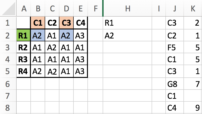
Now, if we wanted to look up what a combination of R1 and C1 gives us, that would be a simple INDEX MATCH MATCH.
But what if we know R1, A2, and want the function to return C1, C3? How do you do this "reverse search"?
Please help
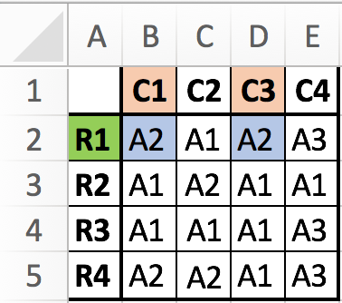
Consider this table:
Now, if we wanted to look up what a combination of R1 and C1 gives us, that would be a simple INDEX MATCH MATCH.
But what if we know R1, A2, and want the function to return C1, C3? How do you do this "reverse search"?
Please help