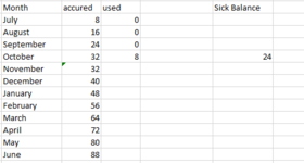
Jamie alexander
New Member
- Joined
- Dec 13, 2021
- Messages
- 8
- Office Version
- 2019
- Platform
- Windows
Your sick balance should be increasing every month ie, time you accrue another 8hrs, minus any used.
I would like to create a spread for sick accrue and used. The employees accrue 8 hours each month. I have attached what I have but missing a step.
Your sick balance should be increasing every month ie, time you accrue another 8hrs, minus any used.
PTO Fellow's.xlsx | |||||||||
---|---|---|---|---|---|---|---|---|---|
C | D | E | F | G | H | I | |||
34 | PTO | Sick time and accure 8 hour each month | |||||||
35 | Month | accured | used | ||||||
36 | July | 8 | 8 | ||||||
37 | August | 8 | 0 | ||||||
38 | September | 16 | 0 | ||||||
39 | October | 24 | 8 | ||||||
40 | November | 24 | |||||||
41 | December | 32 | |||||||
42 | January | 40 | |||||||
43 | February | 48 | |||||||
44 | March | 56 | |||||||
45 | April | 64 | |||||||
46 | May | 72 | |||||||
47 | June | 80 | |||||||
Desai |
Cell Formulas | ||
---|---|---|
Range | Formula | |
D37:D47 | D37 | =D36-E36+8 |
I have the following worksheet that I started for PTO and Sick :
PTO Fellow's.xlsx
C D E F G H I 34 PTO Sick time and accure 8 hour each month 35 Month accured used 36 July 8 8 37 August 8 0 38 September 16 0 39 October 24 8 40 November 24 41 December 32 42 January 40 43 February 48 44 March 56 45 April 64 46 May 72 47 June 80 Desai
Cell Formulas Range Formula D37:D47 D37 =D36-E36+8
Book1.xlsm | |||||
---|---|---|---|---|---|
C | D | E | |||
35 | Month | accrued | used | ||
36 | July | 0 | 8 | ||
37 | August | 8 | 0 | ||
38 | September | 16 | 0 | ||
39 | October | 16 | 8 | ||
40 | November | 24 | |||
41 | December | 32 | |||
42 | January | 40 | |||
43 | February | 48 | |||
44 | March | 56 | |||
45 | April | 64 | |||
46 | May | 72 | |||
47 | June | 80 | |||
Sheet2 |
Cell Formulas | ||
---|---|---|
Range | Formula | |
D36 | D36 | =8-E36 |
D37:D47 | D37 | =+D36+8-E37 |
sick time.xlsx | |||||||||
---|---|---|---|---|---|---|---|---|---|
A | B | C | D | E | F | G | |||
1 | Month | Accrured | Used | Balance | Award Time? | Sick time per month | 8 | ||
2 | January | 0 | 0 | put yes in E for when time is awarded | |||||
3 | February | 0 | 0 | ||||||
4 | March | 0 | 0 | ||||||
5 | April | 0 | 0 | ||||||
6 | May | 0 | 0 | ||||||
7 | June | 0 | 0 | ||||||
8 | July | 0 | 0 | ||||||
9 | August | 0 | 0 | ||||||
10 | September | 0 | 0 | ||||||
11 | October | 0 | 0 | ||||||
12 | November | 0 | 0 | ||||||
13 | December | 0 | 0 | ||||||
14 | Total | 0 | 0 | 0 | |||||
Sheet1 |
Cell Formulas | ||
---|---|---|
Range | Formula | |
B2:B13 | B2 | =IF([@[Award Time?]]="Yes",G$1,0) |
D2 | D2 | =B2-C2 |
D3:D13 | D3 | =B3-C3+D2 |
B14 | B14 | =SUBTOTAL(109,[Accrured]) |
C14 | C14 | =SUBTOTAL(109,[Used]) |
D14 | D14 | =SUBTOTAL(109,[Balance]) |
Cells with Data Validation | ||
---|---|---|
Cell | Allow | Criteria |
E2:E13 | List | Yes |
So My calendar year is July to June and each month they get 8 of sick time. So the award time column I would put 8?
sick time.xlsx
A B C D E F G 1 Month Accrured Used Balance Award Time? Sick time per month 8 2 January 0 0 put yes in E for when time is awarded 3 February 0 0 4 March 0 0 5 April 0 0 6 May 0 0 7 June 0 0 8 July 0 0 9 August 0 0 10 September 0 0 11 October 0 0 12 November 0 0 13 December 0 0 14 Total 0 0 0 Sheet1
Cell Formulas Range Formula B2:B13 B2 =IF([@[Award Time?]]="Yes",G$1,0) D2 D2 =B2-C2 D3:D13 D3 =B3-C3+D2 B14 B14 =SUBTOTAL(109,[Accrured]) C14 C14 =SUBTOTAL(109,[Used]) D14 D14 =SUBTOTAL(109,[Balance])
Cells with Data Validation Cell Allow Criteria E2:E13 List Yes