Sum with condition until value reached and return another cell on same line

Vinch

New Member
Joined
Sep 6, 2023
Messages
1
Office Version
  1. 365
Platform
  1. Windows
Hello,

I have two sheets in my file:
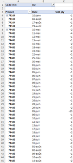
- a table with the amount of sales, per day, for each product (sales per day)
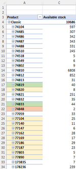
- a second table with each product and the available stock (available stock)

For each product that is availble in stock, I would like to return the amount of days that is took to sell the same quantity that is available in stock.

I already tried a formula as: MATCH(C5,SUBTOTAL(9,OFFSET($C$4,,,ROW($C$7:$C$1000)-ROW($C$4))),1)
where C5 is in my sheet "available stock" and the range "$C$7:$C$1000" is in my sheet "sales per day. → this seems to work but it doesn't take into account my product reference... I cannot find any way to do so :(

Do you have a better way to calculate this?
I already spent hours on google and other forums but I couldn't find any formula that could work.

Thank you!
 

Attachments

  • Available stock.png
    Available stock.png
    18.7 KB · Views: 3
  • Sales per day.png
    Sales per day.png
    20.2 KB · Views: 3

Excel Facts

How to fill five years of quarters?
Type 1Q-2023 in a cell. Grab the fill handle and drag down or right. After 4Q-2023, Excel will jump to 1Q-2024. Dash can be any character.
I made up a small set of data and found a way to get the estimated days of stock. I think it should get you started...
Book1.xlsx
ABCDEFGHIJK
1ProductDate SoldQty SoldProductQty StockProduct to EvaluateC
2A8/27/202314A80
3B8/4/20238B75
4C8/29/20235C120ProductDate SoldQty SoldRunning Total
5A8/16/20233C8/29/202355
6B8/11/20235C8/22/2023611
7C8/22/20236C8/22/2023718
8A8/19/20238C8/22/20231028
9B8/28/202312C8/20/20231038
10C8/20/202310C8/19/20231452
11A8/12/20235C8/8/2023860
12B8/10/20234C8/5/2023666
13C8/22/20237C8/3/20231177
14A8/15/20235C8/3/2023986
15B8/12/20239
16C8/3/202311
17A8/4/20234Qty Match# of DaysDays of Stock
18B8/11/202311862737
19C8/8/20238
20A8/8/20235
21B8/28/20239
22C8/22/202310
23A8/18/20237
24B8/3/202310
25C8/5/20236
26A8/16/20236
27B8/15/20237
28C8/3/20239
29A8/2/20233
30B8/2/202311
31C8/19/202314
Sheet4
Cell Formulas
RangeFormula
H5:J14H5=LET(filt,FILTER(Table2,Table2[Product]=J1),SORTBY(filt,INDEX(filt,,2),-1))
K5:K14K5=SUM($J$5:J5)
H18H18=INDEX(K5:K14,MATCH(VLOOKUP(J1,$E$2:$F$4,2,FALSE),K5:K14,1))
I18I18=I5-INDEX(I5:I14,MATCH(VLOOKUP(J1,$E$2:$F$4,2,FALSE),K5:K14,1))+1
J18J18=ROUNDDOWN(VLOOKUP(J1,$E$2:$F$4,2,FALSE)/H18*I18,0)
Dynamic array formulas.
Cells with Data Validation
CellAllowCriteria
J1List=$E$2:$E$4

Change the value in J1 to evaluate the other products. This could probably be all smashed together into a single formula with some effort.

Hope it helps,

Doug
 
Upvote 0

Forum statistics

Threads
1,215,093
Messages
6,123,068
Members
449,091
Latest member
remmuS24

We've detected that you are using an adblocker.

We have a great community of people providing Excel help here, but the hosting costs are enormous. You can help keep this site running by allowing ads on MrExcel.com.
Allow Ads at MrExcel

Which adblocker are you using?

Disable AdBlock

Follow these easy steps to disable AdBlock

1)Click on the icon in the browser’s toolbar.
2)Click on the icon in the browser’s toolbar.
2)Click on the "Pause on this site" option.
Go back

Disable AdBlock Plus

Follow these easy steps to disable AdBlock Plus

1)Click on the icon in the browser’s toolbar.
2)Click on the toggle to disable it for "mrexcel.com".
Go back

Disable uBlock Origin

Follow these easy steps to disable uBlock Origin

1)Click on the icon in the browser’s toolbar.
2)Click on the "Power" button.
3)Click on the "Refresh" button.
Go back

Disable uBlock

Follow these easy steps to disable uBlock

1)Click on the icon in the browser’s toolbar.
2)Click on the "Power" button.
3)Click on the "Refresh" button.
Go back
Back
Top