Formula or VBA to increase a cell value based off another cell.

[Flexi1]

Hi

I need some help and I hope I am explaining this correctly, I have attached a photo of my spreadsheet and I need
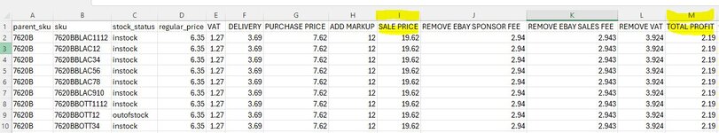
to increase the value of column (M) so that each value has a minimum profit of 2.50

Column (M) is determined by column (I) so I need something that will adjust column (I) until the value
in column (M) reaches 2.50.

Any figures in column (M) that are above 2.50 need to be skipped as they are already good.

Basically I need the sale price in column (I) to increase so that the profit is a min of 2.50 on all items that currently fall below that amount, the full spreadsheet has 100,00 rows
( Column (I) and (M) have formulas already applied to get their totals, not sure if that matters)

 

[Joe4]

I think we need to see what the current formulas in there columns are!
Can you please post those?

It would be really helpful if you also posted the data in a format that we can copy and paste in Excel (not an image).
MrExcel has a tool called “XL2BB” that lets you post samples of your data that will allow us to copy/paste it to our Excel spreadsheets, so we can work with the same copy of data that you are. Instructions on using this tool can be found here: XL2BB Add-in

Note that there is also a "Test Here” forum on this board. This is a place where you can test using this tool (or any other posting techniques that you want to test) before trying to use those tools in your actual posts.

 

[Flexi1]

Ok I will do this now and see if I can get it to work

 

[Flexi1]

RALA SAMPLE SPREADHSEET 2.xlsx
	A	B	C	D	E	F	G	H	I	J	K	L	M
1	parent_sku	sku	stock_status	regular_price	VAT	DELIVERY	PURCHASE PRICE	ADD MARKUP	SALE PRICE	REMOVE EBAY SPONSOR FEE	REMOVE EBAY SALES FEE	REMOVE VAT	TOTAL PROFIT
2	7620B	7620BBLAC1112	instock	6.35	1.27	3.69	7.62	12	19.62	2.943	2.943	3.924	2.19
3	7620B	7620BBLAC12	instock	6.35	1.27	3.69	7.62	12	19.62	2.943	2.943	3.924	2.19
4	7620B	7620BBLAC34	instock	6.35	1.27	3.69	7.62	12	19.62	2.943	2.943	3.924	2.19
5	7620B	7620BBLAC56	instock	6.35	1.27	3.69	7.62	12	19.62	2.943	2.943	3.924	2.19
6	7620B	7620BBLAC78	instock	6.35	1.27	3.69	7.62	12	19.62	2.943	2.943	3.924	2.19
7	7620B	7620BBLAC910	instock	6.35	1.27	3.69	7.62	12	19.62	2.943	2.943	3.924	2.19
8	7620B	7620BBOTT1112	instock	6.35	1.27	3.69	7.62	12	19.62	2.943	2.943	3.924	2.19
9	7620B	7620BBOTT12	outofstock	6.35	1.27	3.69	7.62	12	19.62	2.943	2.943	3.924	2.19
10	7620B	7620BBOTT34	instock	6.35	1.27	3.69	7.62	12	19.62	2.943	2.943	3.924	2.19
RALA SAMPLE SPREADHSEET

Cell Formulas
Range	Formula
I2:I10	I2	=G2+H2
J2:J10	J2	=I2*0.15
K2:K10	K2	=I2*0.15
L2:L10	L2	=I2*0.2
M2:M10	M2	=I2-G2-J2-K2-L2
G2:G10	G2	=D2+E2

 

[Joe4]

Thank you for that.

Can you pick one of the rows, and walk us through the logic of how we are to increase column M to $2.50?
We need to know which columns we are allowed to increase/decrease in order to in order to get there, as there are different options.

 

[Flexi1]

I need to increase the sale price (I) so that the total profit (M) shows as 2.50, all other rows will stay the same and only (i) can change

Obviously I would do this manually but there are 100,000 rows with different data in (I) for each one.

Any rows where (M) is already above 2.50 need to be left alone.

 

[Joe4]

I need to increase the sale price (I) so that the total profit (M) shows as 2.50, all other rows will stay the same and only (i) can change

Obviously I would do this manually but there are 100,000 rows with different data in (I) for each one.

Any rows where (M) is already above 2.50 need to be left alone.

But column I is not a hard-coded value. It is a formula, adding up columns G (Purchase Price) and H (Markup).

And column G (Purchase Price) is a formula adding up columns D (regular_price) and E (VAT).

So, I will ask you once again, which columns (and I should stress I mean hard-coded columns, not formula columns) are we allowed to change to increase your profit?
It looks like columns D, E, F and H are the only hard-coded columns.

 

[Flexi1]

Sorry I see what has happened there, I was meant to remove the formula for that column when I created the spreadsheet to upload here, looks like I forgot. The figure in (I) isn't meant to have the formula in there.

 

[Flexi1]

RALA SAMPLE SPREADHSEET 2.xlsx
	A	B	C	D	E	F	G	H	I	J	K	L	M
1	parent_sku	sku	stock_status	regular_price	VAT	DELIVERY	PURCHASE PRICE	ADD MARKUP	SALE PRICE	REMOVE EBAY SPONSOR FEE	REMOVE EBAY SALES FEE	REMOVE VAT	TOTAL PROFIT
2	7620B	7620BBLAC1112	instock	6.35	1.27	3.69	7.62	12	19.62	2.943	2.943	3.924	2.19
3	7620B	7620BBLAC12	instock	6.35	1.27	3.69	7.62	12	19.62	2.943	2.943	3.924	2.19
4	7620B	7620BBLAC34	instock	6.35	1.27	3.69	7.62	12	19.62	2.943	2.943	3.924	2.19
5	7620B	7620BBLAC56	instock	6.35	1.27	3.69	7.62	12	19.62	2.943	2.943	3.924	2.19
6	7620B	7620BBLAC78	instock	6.35	1.27	3.69	7.62	12	19.62	2.943	2.943	3.924	2.19
7	7620B	7620BBLAC910	instock	6.35	1.27	3.69	7.62	12	19.62	2.943	2.943	3.924	2.19
8	7620B	7620BBOTT1112	instock	6.35	1.27	3.69	7.62	12	19.62	2.943	2.943	3.924	2.19
9	7620B	7620BBOTT12	outofstock	6.35	1.27	3.69	7.62	12	19.62	2.943	2.943	3.924	2.19
10	7620B	7620BBOTT34	instock	6.35	1.27	3.69	7.62	12	19.62	2.943	2.943	3.924	2.19
RALA SAMPLE SPREADHSEET

Cell Formulas
Range	Formula
J2:J10	J2	=I2*0.15
K2:K10	K2	=I2*0.15
L2:L10	L2	=I2*0.2
M2:M10	M2	=I2-G2-J2-K2-L2
G2:G10	G2	=D2+E2

 

[NateSC]

My 2 cents, I would add some columns so you can have some flexibility on the Target Profit (My column O). If you are happy with the results in P, then you can copy that column and Paste Special - Values back into I. And I threw in some conditional formatting on the Profit column so you can see which ones fall below the target. This method lets you preview the changes that will be made before you replace the existing data.
(I had created the data and formulas from your first picture so my column headings are messed up. I changed data in G and H to test different results.)

Book1
	A	B	C	D	E	F	G	H	I	J	K	L	M	N	O	P	Q
1									price				profit		Target Profit	Updated Sale Price	Updated Profit
2	7620B	7620BBLAC1112	instock	6.35	1.27	3.69	7.62	12	19.62	2.94	2.943	3.924	2.19		2.50	19.93	2.50
3	7620B	qwerty	instock	6.35	1.27	3.69	7.62	13	20.62	2.94	2.943	3.924	3.19			20.62	3.19
4	7620B	asdfgh	instock	6.35	1.27	3.69	8	10	18.00	2.94	2.943	3.924	0.19			20.31	2.50
Sheet1

Cell Formulas
Range	Formula
P2:P4	P2	=IF(M2<$O$2,($O$2-M2)+I2,I2)
Q2:Q4	Q2	=P2-L2-K2-J2-G2

Cells with Conditional Formatting
Cell	Condition		Cell Format	Stop If True
M2:M4	Expression	=M2<$O$2	text	NO