SUMIFS formula returning 0

[Zazzy44]

Hi,

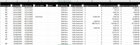
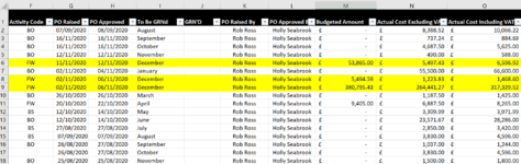
I am using the formula =SUMIFS(POs!O2:O18,POs!I2:I18,FW!B6,POs!F2:F18,FW!B3) to try to total costs by month by budget code in a finance spreadsheet. As far as I am concerned there are totals in the range POs!O2:O18 that match the criteria, but the formula is just returning 0 and it's driving me nuts! What am I doing wrong? Screenshots of the 2 tabs below...

& here's the tab it's pulling from with the rows I think should be being picked up highlighted...

Thank you in advance!!

 

[Peter_SSs]

Welcome to the MrExcel board!

Very hard to tell from a picture. Suggest you investigate XL2BB for providing sample data to make it easier for helpers by not having to manually type out sample data to test with & ensure we have the same data you have.

However, a couple of possible culprits
- Trailing (or leading) spaces in cells that appear the same.
- Month names could be text in one place and date (number) formatted to only show month in another place

 

[mohadin]

See if this what you want

=SUMIFS(POs!$O$2:$O$18,POs!$I$2:$I$18,$B$2:$B$18,POs!$P$2:$P$18,$B$3)

 

[Zazzy44]

Thanks, I've installed XL2BB and this is what it's giving me. There are no spaces, the months are formatted as text & adding $ signs just caused something weird to happen...

Example PO tracker.xlsx
	K
7
POs

 

[Peter_SSs]

I've installed XL2BB and this is what it's giving me.

You need to select the range you want to display before you click 'Capture Range'

.. and we will probably need to see the extract from each of the two sheets, not just one.

 

[Zazzy44]

Sorry, can't work out to select both sheets at once. This is the sheet containing the formula

Example PO tracker.xlsx
	B	C	D	E	F
2
3	FW	Month Budget	Actual Spend	Variance #	Variance %
4	October
5	November
6	December		0
7	January
8	February
9	March
10	April
11	May
12	June
13	July
14	August
15	September
16	Totals
17
FW

Cell Formulas
Range	Formula
D6	D6	=SUMIFS(POs!O2:O18,POs!I2:I18,FW!B6,POs!F2:F18,FW!B3)

And this is where it's pulling from

Example PO tracker.xlsx
	A	B	C	D	E	F	G	H	I	J	K	L	M	N	O	P
1	Product	Supplier	Item Description	Quantity	Date Required	Activity Code	PO Raised	PO Approved	To Be GRNd	GRN'D	PO Raised By	PO Approved By	Budgeted Amount	Actual Cost Excluding VAT	Actual Cost Including VAT	PO Number
2	Lottery			1	19/10/2020	BO	07/09/2020	08/09/2020					£ -	£ 8,388.52	£ 10,066.22	1500/3417930
3	Lottery			1	16/11/2020	BO	16/11/2020	16/11/2020					£ -	£ 737.24	£ 884.69	1500/3421441
4	Lottery			1	16/11/2020	BO	16/11/2020	16/11/2020					£ -	£ 4,687.50	£ 5,625.00	1500/3421440
5	Lottery			1	12/11/2020	BO	12/11/2020	12/11/2020					£ -	£ 490.00	£ 588.00	1500/3421279
6	Lottery			1	12/11/2020	FW	11/11/2020	12/11/2020	December				£ 53,865.00	£ 5,497.43	£ 6,596.92	1500/3421277
7	Lottery			1	02/11/2020	BO	02/11/2020	04/11/2020					£ -	£ 55,500.00	£ 66,600.00	1500/3420992
8	Lottery			1	06/11/2020	FW	02/11/2020	06/11/2020	December				£ 5,494.59	£ 1,223.83	£ 1,468.60	1500/3420991
9	Lottery			1	15/11/2020	FW	02/11/2020	06/11/2020	December				£ 380,795.43	£ 264,441.27	£ 317,329.52	1500/3420988
10	Lottery			1	26/10/2020	BO	26/10/2020	26/10/2020					£ -	£ 1,187.50	£ 1,425.00	1500/3420353
11	Lottery			1	01/02/2021	FW	20/10/2020	22/10/2020					£ 9,405.00	£ 6,887.50	£ 8,265.00	1500/3420198
12	Poppy Supporter			1	11/11/2020	BS	12/10/2020	14/10/2020					£ -	£ 3,309.99	£ 3,971.99	1500/3419806
13	Lottery			1	19/10/2020	BO	12/10/2020	14/10/2020					£ -	£ 23,571.67	£ 28,286.00	1500/3419774
14	Poppy Supporter			1	11/11/2020	BS	27/08/2020	27/08/2020					£ -	£ 2,850.00	£ 3,420.00	1500/3417477
15	Poppy Supporter			1	07/09/2020	BS	07/09/2020	07/09/2020					£ -	£ 3,830.00	£ 4,596.00	1500/3417906
16	Lottery			1	01/10/2020	BO	26/08/2020	27/08/2020					£ -	£ 1,037.00	£ 1,244.00	1500/3417505
17	Regular Giving			1	11/11/2020		26/08/2020	27/08/2020					£ -	£ 3,830.00	£ 4,596.00	1500/3417479
18	Lottery			1	01/09/2020	BO	25/08/2020	25/08/2020					£ -	£ 1,500.00	£ 1,800.00	1500/3417366
POs

Cell Formulas
Range	Formula
N3:N6,N8:N13	N3	=O3/1.2
O7	O7	=N7*1.2

did that work?

 

[Peter_SSs]

did that work?

It did, thanks.

I copied your sheets to a blank workbook (using the BB2XL copy button:

& the formula returned the correct result of 325395.04

Does anything change if you select that cell then press F2 and then Enter?
Check that your calculation is not set to manual (File - Options - Formulas)
Check the cell formatting of that formula cell in case there is something unusual

As an aside, it is not a good idea to use the sheet name for cells that are actually on the sheet the formula is in. It should be relating to this current problem but can cause problems if data is to be sorted. so I would change to

=SUMIFS(POs!O2:O18,POs!I2:I18,B6,POs!F2:F18,B3)

or, if you are going to be copying the formula up/down that column you need to add a few $ signs.

=SUMIFS(POs!O$2:O$18,POs!I$2:I$18,B6,POs!F$2:F$18,B$3)