What would be best formula to use to extract data based on dates with a criteria?

PandaRama

New Member
Joined
Sep 6, 2023
Messages
5
Office Version
  1. 365
Platform
  1. Windows
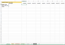
I have an excel where I need to pull in the total hours for a date range (always start on Monday) in my excel tab called 'Dashboard'. I'll be getting the data from the tab 'Budget' but I only want to pull in the number based on the QuickBooks Code I've identified on B1.

So AH3 will equal to AL11 (total 12 hours).

I am unsure which formula would be best to utilize and would appreciate any ideas. My first thought was SUMIF or FILTER but I keep getting an error.
 

Attachments

  • Budget.PNG
    Budget.PNG
    12.6 KB · Views: 20
  • Dashboard.PNG
    Dashboard.PNG
    42.3 KB · Views: 18

Excel Facts

Did you know Excel offers Filter by Selection?
Add the AutoFilter icon to the Quick Access Toolbar. Select a cell containing Apple, click AutoFilter, and you will get all rows with Apple
If your dates will always be in the same order then try the formula in AH8.
If dates could be in different orders between sheets then try the formula in AH3.
Change ranges to match your data.

Sheet 2
Book2
ABAHAIAJAKALAM
1QuickBooks Code: Project Beta
28/7/20238/14/20238/21/20238/28/2023
3Budget (Client)012202040
4Forecast (Internal) 000
5Actuals0
6
7If dates will always be in the same order on each sheet
8Budget (Client)12202040
Sheet2
Cell Formulas
RangeFormula
AH3:AK3AH3=INDEX(Sheet1!$AL$2:$AO$4,MATCH($B$1,Sheet1!$C$2:$C$4,0),MATCH(AH$2,Sheet1!$AL$1:$AO$1,0))
AH8:AK8AH8=FILTER(Sheet1!$AL$2:$AO$4,(Sheet1!$C$2:$C$4=$B$1))
Dynamic array formulas.


Sheet 1
Book2
ABCDEFGHIJKALAMANAO
1CustomerQuickBooks CodeStatusRateTotal BugetTotal Budget8/7/20238/14/20238/21/20238/28/2023
2Client 1Project AActive$
3Client 2Project BetaActive$125$25712202040
4Client 3Project CActive$0
Sheet1
 
Upvote 1
If your dates will always be in the same order then try the formula in AH8.
If dates could be in different orders between sheets then try the formula in AH3.
Change ranges to match your data.

Sheet 2
Book2
ABAHAIAJAKALAM
1QuickBooks Code: Project Beta
28/7/20238/14/20238/21/20238/28/2023
3Budget (Client)012202040
4Forecast (Internal) 000
5Actuals0
6
7If dates will always be in the same order on each sheet
8Budget (Client)12202040
Sheet2
Cell Formulas
RangeFormula
AH3:AK3AH3=INDEX(Sheet1!$AL$2:$AO$4,MATCH($B$1,Sheet1!$C$2:$C$4,0),MATCH(AH$2,Sheet1!$AL$1:$AO$1,0))
AH8:AK8AH8=FILTER(Sheet1!$AL$2:$AO$4,(Sheet1!$C$2:$C$4=$B$1))
Dynamic array formulas.


Sheet 1
Book2
ABCDEFGHIJKALAMANAO
1CustomerQuickBooks CodeStatusRateTotal BugetTotal Budget8/7/20238/14/20238/21/20238/28/2023
2Client 1Project AActive$
3Client 2Project BetaActive$125$25712202040
4Client 3Project CActive$0
Sheet1
Awesome! I'll give this a try
 
Upvote 0
If your dates will always be in the same order then try the formula in AH8.
If dates could be in different orders between sheets then try the formula in AH3.
Change ranges to match your data.

Sheet 2
Book2
ABAHAIAJAKALAM
1QuickBooks Code: Project Beta
28/7/20238/14/20238/21/20238/28/2023
3Budget (Client)012202040
4Forecast (Internal) 000
5Actuals0
6
7If dates will always be in the same order on each sheet
8Budget (Client)12202040
Sheet2
Cell Formulas
RangeFormula
AH3:AK3AH3=INDEX(Sheet1!$AL$2:$AO$4,MATCH($B$1,Sheet1!$C$2:$C$4,0),MATCH(AH$2,Sheet1!$AL$1:$AO$1,0))
AH8:AK8AH8=FILTER(Sheet1!$AL$2:$AO$4,(Sheet1!$C$2:$C$4=$B$1))
Dynamic array formulas.


Sheet 1
Book2
ABCDEFGHIJKALAMANAO
1CustomerQuickBooks CodeStatusRateTotal BugetTotal Budget8/7/20238/14/20238/21/20238/28/2023
2Client 1Project AActive$
3Client 2Project BetaActive$125$25712202040
4Client 3Project CActive$0
Sheet1
What if for example on Sheet 2 I want B2 to = Project A instead of Project Beta. Is there a way to change the range so it's showing the entire table of Sheet 2 (AL2:AO4)?
 
Upvote 0
Seems I might be doing something incorrectly on CELL C3, I keep getting #N/A

Excel Sheet 1 (Tab 1 Called Dashboard)
ABCDEFGHIJKLMN
1QuickBooks Code:Project A
2Total Budget
1/2/2023​
1/9/2023​
1/16/2023​
1/23/2023​
1/30/2023​
2/6/2023​
2/13/2023​
2/20/2023​
2/27/2023​
3/6/2023​
3/13/2023​
3/20/2023​
3Budget (Client)SUM(C3:BB3)
=INDEX(Budget!G1:BF169,MATCH(Dashboard!B1,Budget!B1:B169,0),MATCH(Dashboard!B1,Budget!G1:BF169))
4Forecast (Internal)SUM(C4:BB4)
5ActualsSUM(C5:BB5)

Excel Sheet 1 (Tab 2 Called Budget)
ABCDEFGHIJKLMNOPQ
1QuickBooks CodeStatusRateTotal Buget (Dollar)Total Budget1/2/20231/9/20231/16/20231/23/20231/30/20232/6/20232/13/20232/20/20232/27/20233/6/20233/13/20233/20/2023
2Project ZArchive$ -=[@Rate]*[@[Total Budget]]
=SUM(G2:BF)​
3Project YArchive$ -
0​
4Project 3Archive$ -
0​
5Project 2Archive$ -
0​
6Project 31Archive$ -
0​
7Project 5Archive$ -
0​
8Project hArchive$ -
0​
9Project iArchive$ -
0​
10Project AActive$ 125.00$ 6,000.00
48​
10​
12​
13​
13​
11Project BetaActive$ 125.00$ 32,125.00
257​
12Project CActive$ 125.00$ 1,625.00
13​
5​
1​
4​
3​
 
Upvote 0
I'm taking some guesses at what your actual ranges are.

The first part of the INDEX should be the range of the data you want to return.
INDEX(Budget!G1:BF169 looks like this should be Budget!F2:BF169
The first match should be the rows that fold the project.
MATCH(Dashboard!B1,Budget!B1:B169,0) maybe change to Dashboard!$B$1,Budget!A2:A169,0) Note: the A169 would be the last row in column A that has a project.
The second match would be for your dates
MATCH(Dashboard!B1,Budget!G1:BF169) maybe MATCH(Dashboard!C$2,Budget!$F$2:$BF$169,0)

Also maybe try:
=Filter(Budget!$F$2:$BF$169,Dashboard!$B$1=Budget!$A$2:$A$169)
 
Upvote 1
Solution
I'm taking some guesses at what your actual ranges are.

The first part of the INDEX should be the range of the data you want to return.
INDEX(Budget!G1:BF169 looks like this should be Budget!F2:BF169
The first match should be the rows that fold the project.
MATCH(Dashboard!B1,Budget!B1:B169,0) maybe change to Dashboard!$B$1,Budget!A2:A169,0) Note: the A169 would be the last row in column A that has a project.
The second match would be for your dates
MATCH(Dashboard!B1,Budget!G1:BF169) maybe MATCH(Dashboard!C$2,Budget!$F$2:$BF$169,0)

Also maybe try:
=Filter(Budget!$F$2:$BF$169,Dashboard!$B$1=Budget!$A$2:$A$169)
Thank you! Realized I pasted the wrong formula from my excel as it's more data showing. I'll give this another try!
 
Upvote 0

Forum statistics

Threads
1,215,069
Messages
6,122,954
Members
449,095
Latest member
nmaske

We've detected that you are using an adblocker.

We have a great community of people providing Excel help here, but the hosting costs are enormous. You can help keep this site running by allowing ads on MrExcel.com.
Allow Ads at MrExcel

Which adblocker are you using?

Disable AdBlock

Follow these easy steps to disable AdBlock

1)Click on the icon in the browser’s toolbar.
2)Click on the icon in the browser’s toolbar.
2)Click on the "Pause on this site" option.
Go back

Disable AdBlock Plus

Follow these easy steps to disable AdBlock Plus

1)Click on the icon in the browser’s toolbar.
2)Click on the toggle to disable it for "mrexcel.com".
Go back

Disable uBlock Origin

Follow these easy steps to disable uBlock Origin

1)Click on the icon in the browser’s toolbar.
2)Click on the "Power" button.
3)Click on the "Refresh" button.
Go back

Disable uBlock

Follow these easy steps to disable uBlock

1)Click on the icon in the browser’s toolbar.
2)Click on the "Power" button.
3)Click on the "Refresh" button.
Go back
Back
Top