Text Conditional formatting if cell not equal to another

[Paul Naylor]

Hoping someone can help?

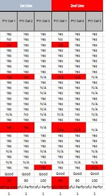
Need to identify some variances in columns of text data . Although multiple columns I don't want to use multiple helper columns and thought easiest & most visually striking way is to use conditional formatting to highlight using a colour any differences in the 2nd column of data.

1st column C3-C47 contains manager call observation results to various questions ( text) and 2nd column G3-G47 contains quality team call observations results to the same set of questions.

All I would like is for any of the answers in the 2nd set of data are not equal to 1st set is for the relevant answer in the 2nd set to be highlighted in a colour.

I've tried to do this with conditional formatting , but all methods I've looked at seem to need an extra column , but with potentially 40 different comparisons spreadsheet will be unusable.

Anyone any ideas of how to do?

E.g. 2 columns of data on call observations answers to a number of questions. One set say in column C is managers observations and 2nd set say in column G is quality teams observations. Need to be able to identify by any differences between the managers observations and

 

[etaf]

would a countif() work

= countif($C$3:$C$47,G3)=0

But i feel maybe a lot more complicated then this , but i'm not really following so not sure why
dont understand this comment

but with potentially 40 different comparisons spreadsheet will be unusable.

A SMALL sample spreadsheet, around 10-20 rows, would help a lot here, with all sensitive data removed, and expected results mocked up and manually entered, with a few notes of explanation.

MrExcel has a tool called “XL2BB” that lets you post samples of your data and will allow us to copy/paste your sample data into our Excel spreadsheets, saving a lot of time.

XL2BB - Excel Range to BBCode

Excel 'mini-sheet' in messages - XL2BB Although experts prefer to read your description and question instead of working in your actual file to solve your problem, there are times that it is difficult to explain an issue without providing actual...

www.mrexcel.com

You can also test to see if it works ok, in the "Test Here" forum.

Test Here

Use this forum to test your signature, learn bbcode, smilies, XL2BB, etc. Threads in this forum are automatically deleted after no replies for seven (7) days

www.mrexcel.com

OR if you cannot get XL2BB to work, or have restrictions on your PC

then put the sample spreadsheet onto a share

I only tend to goto OneDrive, Dropbox or google docs , as I'm never certain of other random share sites and possible virus.
Please make sure you have a representative data sample and also that the data has been desensitised, remember this site is open to anyone with internet access to see - so any sensitive / personal data should be removed

Make sure you set any share or google to share to everyone

 

[Paul Naylor]

Hi eta,

Thanks for your reply. Just to clarify I'm comparing C3 to G3, C4 to G4, C5 to G5...etc , so if say G3 <> C3 I want G3 cell to be coloured Red , but C3 to remain un-coloured.

 

[etaf]

ok,
then
try

=$C3<>$G3
as a rule

for 2007, 2010 , 2013 , 2016 , 2019 or 365 Subscription excel version
Conditional Formatting

Highlight applicable range >>
G3:G47 - Change, reduce or extend the rows to meet your data range of rows

Home Tab >> Styles >> Conditional Formatting
New Rule >> Use a formula to determine which cells to format
Edit the Rule Description: Format values where this formula is true:
=$C3<>$G3

Format [Number, Font, Border, Fill]
choose the format you would like to apply when the condition is true
OK >> OK

Book1
	A	B	C	D	E	F	G	H
1
2
3			b				d
4			c				c
5			1				4
6			2				2
7							1
8			3				3
9
Sheet1

Cells with Conditional Formatting
Cell	Condition		Cell Format	Stop If True
G3:G8	Expression	=$C3<>$G3	text	YES

 

[Paul Naylor]

Hi Etaf, thanks , seen online solution where highlight both columns and use same technique which highlights both columns , but didn't think that by using same process and selecting only the column I want to highlight would work.

Many ...many ..many thanks ..
Knew someone on the forum would know the best approach

 

[etaf]

glad its worked for you
you are welcome

 

[Paul Naylor]

Hi Etaf, Thanks for your solution, but i didnt factor in the fact that I need an additional check to be done . checks to non adjacent columns (CH & CK, CI & CL & CJ & CM , but only if value in the corresponding cell in row 33 = 1 i.e. CH33,CI33,CJ33( values can be 0 or 1 only) and the adjacent value in the corresponding cell <> do I want both cells to highlight in "Red" , formulas ( see below) using appear to work for this example,

Apply to Range:
CH5:CH32,CK5:CK32

Rule Type:
Formula

Format All Values Where Formula is True:
=IF(AND($SCH33,1),$CH5<>$CK5)

But not other instances where check digit in row 33 =0

Apply to Range:
K5:K32,N5:N32

Rule Type:
Formula

Format All Values Where Formula is True:
=IF(AND($K33,1),$K5<>$N5)

 

[etaf]

sorry, not sure i follow, 1 of the images will not open and to be honest, not really a good way to show the data - as i have to type it all in...... and cannot see any columns or row references - so have no idea how to correlate the wording to the images
BUT as i say , not keen on images

would you use 2XLBB or put on a share like onedrive/dropbox or google sheets

as i say , i'm not really following the explanation of what is needed now

 

[Paul Naylor]

Hi etaf , unable to share via xl2bb , so please find attached dropbox link.

conditional formatting non numerical non matching data.url

Shared with Dropbox

www.dropbox.com

 

[etaf]

in your example I dont see these columns

checks to non adjacent columns (CH & CK, CI & CL & CJ & CM , but only if value in the corresponding cell in row 33 = 1 i.e. CH33,CI33,CJ33( values can be 0 or 1 only)

you have this formula
=IF(AND($B33,1),$B5<>$E5)

To test for row 33 only , if it =1
then you need
B$33=1
that then stops the row changing

and then add to the and

=AND( B$33=1, $B5<>$E5 )
BUT $B5<>$E5
means it will not change columns

so not really following again
column K and N have a zero in row 33

so why are they shown highlighted

also not sure which cells we are comparing now

B with E
C with F

can you manually colour the cells you want to highlight - and explain why - so perhaps i can see what you are now after

this is just applying the formula

=AND( B$33=1, B5<>E5 )
and so as conditional formatting moves across the columns - its checking
B with E
C with F
D with G
etc
which s wrong

Book7.xlsx
	A	B	C	D	E	F	G	H	I	J	K	L	M	N
2
3
4
5		Yes	Yes	Yes	Yes	Yes	Yes		Yes	Yes	Yes	Yes	Yes	--
6		No	Yes	Yes	No	Yes	Yes		Yes	Yes	Yes	Yes	Yes	--
7		No	Yes	Yes	Yes	Yes	Yes		Yes	Yes	No	Yes	Yes	--
8		Yes	Yes	Yes	Yes	Yes	Yes		Yes	Yes	Yes	Yes	Yes	--
9		Yes	Yes	Yes	Yes	Yes	Yes		Yes	No	Yes	Yes	Yes	--
10		Yes	Yes	Yes	Yes	Yes	Yes		No	Yes	Yes	Yes	Yes	--
11		Yes	Yes	Yes	Yes	Yes	Yes		No	No	Yes	No	Yes	--
12		Yes	Yes	Yes	Yes	Yes	Yes		Minor Feedback	Yes	Yes	Minor Feedback	Yes	--
13		Yes	Yes	N/A	N/A	N/A	N/A		N/A	N/A	N/A	N/A	N/A	--
14		Yes	Yes	Yes	Yes	Yes	Yes		No	Yes	No	No	Yes	--
15		Yes	Yes	N/A	Yes	Yes	N/A		Yes	Yes	Yes	Yes	Yes	--
16		Yes	Yes	N/A	Yes	Yes	N/A		N/A	Yes	Yes	N/A	Yes	--
17		Yes	Yes	Yes	Yes	Yes	Yes		Yes	Yes	Yes	Yes	Yes	--
18		Yes	Yes	N/A	Yes	Yes	N/A		Yes	Yes	Yes	Yes	Yes	--
19		Yes	Yes	N/A	Yes	Yes	N/A		No	No	No	N/A	No	--
20		N/A	No	N/A	N/A	No	N/A		N/A	No	No	No	No	--
21		Yes	Yes	Yes	Yes	Yes	Yes		No	Yes	No	No	Yes	--
22		Yes	Yes	N/A	N/A	N/A	N/A		N/A	N/A	N/A	N/A	N/A	--
23		Yes	Yes	Yes	Yes	Yes	Yes		Yes	Yes	Yes	Yes	Yes	--
24		Yes	Yes	Yes	Yes	Yes	Yes		Yes	Yes	Minor Feedback	Yes	Yes	--
25		Yes	Yes	Yes	Yes	Yes	Yes		Yes	Yes	Minor Feedback	Yes	Yes	--
26		N/A	Yes	N/A	N/A	Yes	N/A		N/A	Yes	N/A	N/A	N/A	--
27		Yes	Yes	Yes	Yes	Yes	Yes		Yes	Yes	Yes	Yes	Yes	--
28		N/A	N/A	N/A	N/A	N/A	N/A		N/A	N/A	N/A	N/A	N/A	--
29		Yes	Yes	Yes	Yes	Yes	N/A		N/A	Yes	Yes	Yes	Yes	--
30		Good	Good	Good	Good	Good	Good		Development	Good	Poor	Development	Good	--
31		20	90	100	90	90	100		0	45	0	0	65	--
32		Not meeting expectation	Successful Performance	Successful Performance	Successful Performance	Successful Performance	Successful Performance		Not meeting expectation	Not meeting expectation	Not meeting expectation	Not meeting expectation	Inconsistent / Developing performance	--
33		1	1	1	1	1	1		1	1	0	1	1	0
Sheet1 (2)

Cells with Conditional Formatting
Cell	Condition		Cell Format	Stop If True
B5:N32	Expression	=AND(B$33=1, B5<>E5 )	text	YES

dropbox link only stays a few days , before i delete

Dropbox - File Deleted - Simplify your life

www.dropbox.com