Traffic Light System for Dates

[CarmsT]

Hiya everyone!!

Bit of a young buck who for the life of me cannot get this traffic light system to work on an excel spreadsheet! I have tried every forum method and it just wont work!
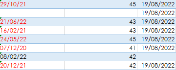
Basically I am data managing patient data and for example I am checking the dates everyone last had their bloods taken. If its within the year 2022 it would be Green. If it was last year Red. And if i have invited them in to have a blood test on for example today - yellow so im aware whos been invited.

Please help! I cant wrap my head around it at all!

 

[jasonb75]

If its within the year 2022 it would be Green. If it was last year Red.

Just a quick check on exact requirement here, should it be calendar year or last 12 months (the way that you have asked your question implies that a blood test carried out in mid December would be valid for less than 1 month, yet one carried out in early January would be valid for almost 12 months

 

[CarmsT]

Just a quick check on exact requirement here, should it be calendar year or last 12 months (the way that you have asked your question implies that a blood test carried out in mid December would be valid for less than 1 month, yet one carried out in early January would be valid for almost 12 months

Also where ive confused myself with the coding of it all sorry! Last 12 months Sorry!

 

[jasonb75]

Also where ive confused myself with the coding of it all

We've all been there and done that. I would doubt the honesty of anyone who says that they haven't.

I've done a quick example for you with some random dates, is this anything close to what you need?

Book1
	A	B	C
1	Last test		Invite
2	03/07/2021
3	20/02/2022
4	09/12/2021
5	11/06/2021
6	26/09/2021
7	20/10/2021
8	10/12/2021
9	08/03/2022
10	12/01/2022
11	26/08/2022
12	24/11/2021
13	24/08/2021
14	10/09/2021		13/09/2022
15	04/07/2021
16	23/05/2021		13/09/2022
17	28/05/2022
18	28/09/2021
19	02/06/2022
20	05/03/2022
21	23/06/2021
22	05/08/2022
23	19/07/2022
24	19/04/2022
Sheet6

Cells with Conditional Formatting
Cell	Condition		Cell Format	Stop If True
A2:A24	Expression	=C2=TODAY()	text	YES
A2:A24	Expression	=A2<TODAY()-365	text	YES
A2:A24	Expression	=A2<TODAY()	text	NO

 

[CarmsT]

YEs exactly that! How do I do that in a Dummies guide?

 

[jasonb75]

How do I do that in a Dummies guide?

I'm never very good at doing these but I'll give it a go,

First, you need to select the range of dates that you want to highlight starting from the top left corner, so from A2 down to A24 in my example sheet.
Next go to the conditional formatting manager, on the Excel ribbon that is Home > Conditional Formatting >Manage rules.

Note that anywhere I've used A2 in the formulas, you will need to use the top left cell of the date range that you have selected (if different).
Where I have used C2 in a formula, you will need to use the cell that contains the Invite Date relative to A2 (doesn't matter if the cell is blank at the moment).

The Next step is to go to New Rule > Use a formula to determine which cells to format.
In the box labelled Format values where this formula is true: enter the bottom formula from the example that I provided earlier (Green highlight).
Click on the Format button below the box that you entered the formula into, then go to the Font tab and click the Color dropdown. Choose your desired shade of green, then click OK twice.

Repeat the steps in the 3 lines above for the Yellow highlight, then the Red highlight using the other 2 formulas from my earlier post.

Make sure that the Stop if True boxes are ticked for the Red and Yellow rules (green doesn't need it). Then click Apply.

You should now see the formatting applied to the sheet behind the pop up box. If all is good then click OK and you're done.

Hopefully I haven't missed any steps but if it looks wrong, please take a screen capture showing as much of the screen as possible without compromising any private / confidential details. Ideally, I need to see the box where you have just set up the 3 formatting rules and the dates in the sheet behind. If you need to trim the top or left side off of the screen capture then I will need to know exactly which rows an columns are visible in the image.

 

[CarmsT]

It didnt work! I have tried a few times and it just doesnt seem to like it

 

[jasonb75]

What is it doing, or not doing? Are you getting any kind of error message?