Hi all,
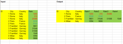
I have a table that looks like the below "Input" and i want to transpose it into a structure like the "Output"
I need to take the unique values in the column "ID". And print it as once even how many time it appears the column till "country" should print once and the values in the "Rate" column should be print in rows until in available for the same "ID". when the value in the "ID" column changes, it the respected values for the next "ID" should start a print in the next row.
Please see the image for reference.
Thanks in advance
")


