Transpose using formulas based on condition

[Sumit_123]

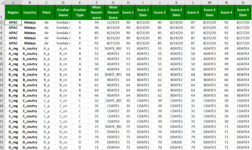
Hi, I have a situation where in I have data where the hierarchy goes as follows
Region>Country>Plant>crusher Name>Machine Score>Machine score check date.

is there a way to transpose the score 1 date below the most recent score column and the date next to it using formulas and likewise for other columns for score 3 date and etc..?
The catch is that the columns from A:E should be repeated for Score1 and date and likewise for score2 and date .

 

[cmowla]

If I am understanding you correctly, yes if you use some math! But you have to have an index column (just an extra column counting). And of course the table that you want to see transposes in needs to be separate from the original data table. (And for this to work the index column must start at 2. But the table can be moved around in the sheet . . . but the two tables need to start on the same row, so I meant move both tables around on the sheet.)

Blank33.xlsb
	A	B	C	D	E	F	G	H	I	J	K	L	M	N	O	P	Q	R	S	T	U	V	W	X
1	Region	Country	Plant	Crusher Name	Crusher Type	Most Recent score	Most Recent Score Date		Region	Country	Plant	Crusher Name	Crusher Type	Most Recent score	Most Recent Score Date	Score 1	Score 1 Date	Score 2	Score 2 Date	Score 3	Score 3 Date	Score 4	Score 4 Date	INDEX COLUMN
2	APAC	Malays	Air	Svedala J	X	94	12/4/2021		APAC	Malays	Air	Svedala J	X	94	12/4/2021	90	8/23/2020	85	8/24/2020	87	8/25/2020	92	8/27/2020	2
3	APAC	Malays	Air	Svedala J	X	90	8/23/2020		A_reg	A_coutry	A_p	A_cn	A	52	ADATE_REC	53	ADATE1	55	ADATE2	50	ADATE3	49	ADATE4	3
4	APAC	Malays	Air	Svedala J	X	85	8/24/2020		B_reg	B_coutry	B_p	B_cn	B	61	BDATE_REC	64	BDATE1	62	BDATE2	64	BDATE3	66	BDATE4	4
5	APAC	Malays	Air	Svedala J	X	87	8/25/2020		C_reg	C_coutry	C_p	C_cn	C	32	CDATE_REC	35	CDATE1	39	CDATE2	31	CDATE3	30	CDATE4	5
6	APAC	Malays	Air	Svedala J	X	92	8/27/2020		D_reg	D_coutry	D_p	D_cn	D	72	DDATE_REC	75	DDATE1	70	DDATE2	79	DDATE3	71	DDATE4	6
7	A_reg	A_coutry	A_p	A_cn	A	52	ADATE_REC																	7
8	A_reg	A_coutry	A_p	A_cn	A	53	ADATE1																	8
9	A_reg	A_coutry	A_p	A_cn	A	55	ADATE2																	9
10	A_reg	A_coutry	A_p	A_cn	A	50	ADATE3																	10
11	A_reg	A_coutry	A_p	A_cn	A	49	ADATE4																	11
12	B_reg	B_coutry	B_p	B_cn	B	61	BDATE_REC																	12
13	B_reg	B_coutry	B_p	B_cn	B	64	BDATE1																	13
14	B_reg	B_coutry	B_p	B_cn	B	62	BDATE2																	14
15	B_reg	B_coutry	B_p	B_cn	B	64	BDATE3																	15
16	B_reg	B_coutry	B_p	B_cn	B	66	BDATE4
17	C_reg	C_coutry	C_p	C_cn	C	32	CDATE_REC
18	C_reg	C_coutry	C_p	C_cn	C	35	CDATE1
19	C_reg	C_coutry	C_p	C_cn	C	39	CDATE2
20	C_reg	C_coutry	C_p	C_cn	C	31	CDATE3
21	C_reg	C_coutry	C_p	C_cn	C	30	CDATE4
22	D_reg	D_coutry	D_p	D_cn	D	72	DDATE_REC
Sheet8 (3)

Cell Formulas
Range	Formula
F2:F22	F2	=SWITCH(MOD(ROW()-2,5),0,INDEX($N$2:$N$6,MATCH(FLOOR((ROW()+3)/5,1)+1,$X$2:$X$6,0),0),1,INDEX($P$2:$P$6,MATCH(FLOOR((ROW()+3)/5,1)+1,$X$2:$X$6,0),0),2,INDEX($R$2:$R$6,MATCH(FLOOR((ROW()+3)/5,1)+1,$X$2:$X$6,0),0),3,INDEX($T$2:$T$6,MATCH(FLOOR((ROW()+3)/5,1)+1,$X$2:$X$6,0),0),4,INDEX($V$2:$V$6,MATCH(FLOOR((ROW()+3)/5,1)+1,$X$2:$X$6,0),0))
G2:G22	G2	=SWITCH(MOD(ROW()-2,5),0,INDEX($O$2:$O$6,MATCH(FLOOR((ROW()+3)/5,1)+1,$X$2:$X$6,0),0),1,INDEX($Q$2:$Q$6,MATCH(FLOOR((ROW()+3)/5,1)+1,$X$2:$X$6,0),0),2,INDEX($S$2:$S$6,MATCH(FLOOR((ROW()+3)/5,1)+1,$X$2:$X$6,0),0),3,INDEX($U$2:$U$6,MATCH(FLOOR((ROW()+3)/5,1)+1,$X$2:$X$6,0),0),4,INDEX($W$2:$W$6,MATCH(FLOOR((ROW()+3)/5,1)+1,$X$2:$X$6,0),0))
A2:E22	A2	=INDEX($I$2:$M$6,MATCH(FLOOR((ROW()+3)/5,1)+1,$X$2:$X$6,0),0)
Dynamic array formulas.

 

[Sumit_123]

Thankyou so much for replying. The solution you provided is exactly what I am looking for but I am not very much advanced in excel. The situation I have is that I have other columns as well in between which I didn't included in the example above(genuine apologies for this).
Because I am not too much advanced in excel I am failing to understand how should I manipulate or what changes in the formula I should be making to address my situation. Can you please guide me in this situation.
Thanks again

 

[cmowla]

Thankyou so much for replying. The solution you provided is exactly what I am looking for but I am not very much advanced in excel. The situation I have is that I have other columns as well in between which I didn't included in the example above(genuine apologies for this).
Because I am not too much advanced in excel I am failing to understand how should I manipulate or what changes in the formula I should be making to address my situation. Can you please guide me in this situation.
Thanks again

What's better than a video? It's 19 minutes long, but I will walk you through each step (to the best of my ability).

Let me know if you have any further questions. And if you have a question about a specific part of the video, just let me know. (For all others reading, the gist of the video is to make use of Excel table objects.)

 

[Fluff]

Another option

+Fluff 1.xlsm
	A	B	C	D	E	F	G	H	I	J	K	L	M	N	O	P	Q	R
1	Region	Country	Plant	Crusher Name	Crusher Type	abc	def	ghi	Most Recent score	Most Recent Score Date	Score 1	Score 1 Date	Score 2	Score 2 Date	Score 3	Score 3 Date	Score 4	Score 4 Date
2	APAC	Malays	Air	Svedala J	X	Data 1	Data 10	Data 20	94	01/01/2021	90	01/02/2021	85	01/03/2021	87	01/04/2021
3	A_reg	A_coutry	A_p	A_cn	A	Data 2	Data 11	Data 21	52	11/01/2021	53	11/02/2021	55	11/03/2021	50	11/04/2021	49	11/05/2021
4	B_reg	B_coutry	B_p	B_cn	B	Data 3	Data 12	Data 22	61	21/01/2021	64	21/02/2021	62	21/03/2021	64	21/04/2021	66	21/05/2021
5	C_reg	C_coutry	C_p	C_cn	C	Data 4	Data 13	Data 23	32	31/01/2021	35	03/03/2021	39	31/03/2021
6	D_reg	D_coutry	D_p	D_cn	D	Data 5	Data 14	Data 24	72	10/02/2021	75	13/03/2021	70	10/04/2021	79	11/05/2021	71	10/06/2021
7
8
9
10
11
12
13
14	APAC	Malays	Air	Svedala J	X	Data 1	Data 10	Data 20	94	01/01/2021
15	APAC	Malays	Air	Svedala J	X	Data 1	Data 10	Data 20	90	01/02/2021
16	APAC	Malays	Air	Svedala J	X	Data 1	Data 10	Data 20	85	01/03/2021
17	APAC	Malays	Air	Svedala J	X	Data 1	Data 10	Data 20	87	01/04/2021
18	A_reg	A_coutry	A_p	A_cn	A	Data 2	Data 11	Data 21	52	11/01/2021
19	A_reg	A_coutry	A_p	A_cn	A	Data 2	Data 11	Data 21	53	11/02/2021
20	A_reg	A_coutry	A_p	A_cn	A	Data 2	Data 11	Data 21	55	11/03/2021
21	A_reg	A_coutry	A_p	A_cn	A	Data 2	Data 11	Data 21	50	11/04/2021
22	A_reg	A_coutry	A_p	A_cn	A	Data 2	Data 11	Data 21	49	11/05/2021
23	B_reg	B_coutry	B_p	B_cn	B	Data 3	Data 12	Data 22	61	21/01/2021
24	B_reg	B_coutry	B_p	B_cn	B	Data 3	Data 12	Data 22	64	21/02/2021
25	B_reg	B_coutry	B_p	B_cn	B	Data 3	Data 12	Data 22	62	21/03/2021
26	B_reg	B_coutry	B_p	B_cn	B	Data 3	Data 12	Data 22	64	21/04/2021
27	B_reg	B_coutry	B_p	B_cn	B	Data 3	Data 12	Data 22	66	21/05/2021
28	C_reg	C_coutry	C_p	C_cn	C	Data 4	Data 13	Data 23	32	31/01/2021
29	C_reg	C_coutry	C_p	C_cn	C	Data 4	Data 13	Data 23	35	03/03/2021
30	C_reg	C_coutry	C_p	C_cn	C	Data 4	Data 13	Data 23	39	31/03/2021
31	D_reg	D_coutry	D_p	D_cn	D	Data 5	Data 14	Data 24	72	10/02/2021
32	D_reg	D_coutry	D_p	D_cn	D	Data 5	Data 14	Data 24	75	13/03/2021
33	D_reg	D_coutry	D_p	D_cn	D	Data 5	Data 14	Data 24	70	10/04/2021
34	D_reg	D_coutry	D_p	D_cn	D	Data 5	Data 14	Data 24	79	11/05/2021
35	D_reg	D_coutry	D_p	D_cn	D	Data 5	Data 14	Data 24	71	10/06/2021
36
Lists

Cell Formulas
Range	Formula
A14:H35	A14	=LET(RngA,A2:H6, RngB,I2:R6,Rws,ROWS(RngA),Qty,SEQUENCE(Rws*COLUMNS(RngB)/2,,0),AryA,INDEX(RngA,INT(Qty/Rws)+1,MOD(Qty,Rws)*0+SEQUENCE(,COLUMNS(RngA))),AryB,INDEX(RngB,INT(Qty/Rws)+1,MOD(Qty,Rws)*2+{1,2}),FILTER(AryA,INDEX(AryB,,1)<>""))
I14:J35	I14	=LET(RngB,I2:R6,Rws,ROWS(RngB),Qty,SEQUENCE(Rws*COLUMNS(RngB)/2,,0),AryB,INDEX(RngB,INT(Qty/Rws)+1,MOD(Qty,Rws)*2+{1,2}),FILTER(AryB,INDEX(AryB,,1)<>""))
Dynamic array formulas.

 

[cmowla]

For those who are curious, in the video I set up a design which removed the dynamic array formulas from my first post. In this one minute (follow-up) video (it had to be 20 minutes, I guess! LOL), I show how to remove the one (unnecessary) dynamic array formula (for the table headers display).

So an index column doesn't have to be displayed with this approach, but just used in the Excel Table object where the data is inputted in.

Also, I posted an image rather than using XL2BB because XL2BB does a poor job of representing the formulas in this sheet. So I list the three formulas that are in a cell which (in the videos) I show that I: place them in a cell to the left, filled them right, and then filled all of those down.

(And note that Table5 is in another sheet. Its header row is also on row 1, but either of the "table" of formulas or the Excel table object can be shifted horizontally left or right.)

Formula in A1. Filled right to O1.

=Table5[[#Headers],[Region]]

Formula in A2. Filled right to O2, but then deleted in F2 and G2. (And of course cells with this formula were then filled down.)

=INDEX(Table5[Region],MATCH(FLOOR((ROW()+3)/5,1)+1,Table5[[INDEX]:[INDEX]],0),0)

Formula in F2. Filled right to G2. (And then the two cells were filled down.)

=SWITCH(MOD(ROW()-2,5),0,INDEX(Table5[Most Recent score],MATCH(FLOOR((ROW()+3)/5,1)+1,Table5[[INDEX]:[INDEX]],0),0),1,INDEX(Table5[Score 1],MATCH(FLOOR((ROW()+3)/5,1)+1,Table5[[INDEX]:[INDEX]],0),0),2,INDEX(Table5[Score 2],MATCH(FLOOR((ROW()+3)/5,1)+1,Table5[[INDEX]:[INDEX]],0),0),3,INDEX(Table5[Score 3],MATCH(FLOOR((ROW()+3)/5,1)+1,Table5[[INDEX]:[INDEX]],0),0),4,INDEX(Table5[Score 4],MATCH(FLOOR((ROW()+3)/5,1)+1,Table5[[INDEX]:[INDEX]],0),0))

And speaking of which (I mean "SWITCH"), I guess I should make this completely transferrable to other versions of Office besides 365 if I convert it into a nested IF statement:

=IF(MOD(ROW()-2,5) = 0, INDEX(Table5[Most Recent score],MATCH(FLOOR((ROW()+3)/5,1)+1,Table5[[INDEX]:[INDEX]],0),0),
IF(MOD(ROW()-2,5) = 1,INDEX(Table5[Score 1],MATCH(FLOOR((ROW()+3)/5,1)+1,Table5[[INDEX]:[INDEX]],0),0),
IF(MOD(ROW()-2,5) = 2,INDEX(Table5[Score 2],MATCH(FLOOR((ROW()+3)/5,1)+1,Table5[[INDEX]:[INDEX]],0),0),
IF(MOD(ROW()-2,5) = 3,INDEX(Table5[Score 3],MATCH(FLOOR((ROW()+3)/5,1)+1,Table5[[INDEX]:[INDEX]],0),0),
IF(MOD(ROW()-2,5) = 4,INDEX(Table5[Score 4],MATCH(FLOOR((ROW()+3)/5,1)+1,Table5[[INDEX]:[INDEX]],0),0))))))

 

[Sumit_123]

Thanks a lot for such a detailed video. I am really grateful and thankful to you for doing such a great effort. I was able to understand all of it.
Just one quick question that I had - If i had more scores and date what should i be changing in the formula that you provided (like in the image below)?

As per the image on the left I am getting results for until Score 4 date and then everything is being messed up.

 

[cmowla]

Thanks a lot for such a detailed video. I am really grateful and thankful to you for doing such a great effort. I was able to understand all of it.
Just one quick question that I had - If i had more scores and date what should i be changing in the formula that you provided (like in the image below)?

View attachment 48533

View attachment 48532As per the image on the left I am getting results for until Score 4 date and then everything is being messed up.

You would add to the SWITCH statement.

Following the (long) video's example, let's focus on the Most Recent score column's formula. Once we make a formula for that, we can just fill right to the Most Recent Score Date column to its immediate right.

Right now the Most Recent score formula is the following.

=SWITCH(MOD(ROW()-2,5),
0,INDEX(Table5[Most Recent score],MATCH(FLOOR((ROW()+3)/5,1)+1,Table5[[INDEX]:[INDEX]],0),0),
1,INDEX(Table5[Score 1],MATCH(FLOOR((ROW()+3)/5,1)+1,Table5[[INDEX]:[INDEX]],0),0),
2,INDEX(Table5[Score 2],MATCH(FLOOR((ROW()+3)/5,1)+1,Table5[[INDEX]:[INDEX]],0),0),
3,INDEX(Table5[Score 3],MATCH(FLOOR((ROW()+3)/5,1)+1,Table5[[INDEX]:[INDEX]],0),0),
4,INDEX(Table5[Score 4],MATCH(FLOOR((ROW()+3)/5,1)+1,Table5[[INDEX]:[INDEX]],0),0)
)

We have 0 through 4 = 5 different possibilities (including most recent score and scores 1-4). And we /5 and have ,5 after "MOD(ROW()-2".

In general, this can be rewritten as the following, where X is the number of scores you have (which is also the number of score dates you have) -- including the most recent . . . so in the example above, X=4, because we had 4 scores in the original image).

=SWITCH(MOD(ROW()-2,5),
0,INDEX(Table5[Most Recent score],MATCH(FLOOR((ROW()+X-1)/5,1)+1,Table5[[INDEX]:[INDEX]],0),0),
1,INDEX(Table5[Score 1],MATCH(FLOOR((ROW()+X-1)/5,1)+1,Table5[[INDEX]:[INDEX]],0),0),
2,INDEX(Table5[Score 2],MATCH(FLOOR((ROW()+X-1)/5,1)+1,Table5[[INDEX]:[INDEX]],0),0),
3,INDEX(Table5[Score 3],MATCH(FLOOR((ROW()+X-1)/5,1)+1,Table5[[INDEX]:[INDEX]],0),0),
4,INDEX(Table5[Score 4],MATCH(FLOOR((ROW()+X-1)/5,1)+1,Table5[[INDEX]:[INDEX]],0),0)
)

If we have the most recent score + scores 1-8, then we would have 0 through 8. And we /9 and have ,9 after "MOD(ROW()-2".
(Also write [Score 1] through [Score 8]. Also X-1 = 8-1 = 7 in this case, since we have 8 scores.)

=SWITCH(MOD(ROW()-2,9),
0,INDEX(Table5[Most Recent score],MATCH(FLOOR((ROW()+7)/9,1)+1,Table5[[INDEX]:[INDEX]],0),0),
1,INDEX(Table5[Score 1],MATCH(FLOOR((ROW()+7)/9,1)+1,Table5[[INDEX]:[INDEX]],0),0),
2,INDEX(Table5[Score 2],MATCH(FLOOR((ROW()+7)/9,1)+1,Table5[[INDEX]:[INDEX]],0),0),
3,INDEX(Table5[Score 3],MATCH(FLOOR((ROW()+7)/9,1)+1,Table5[[INDEX]:[INDEX]],0),0),
4,INDEX(Table5[Score 4],MATCH(FLOOR((ROW()+7)/9,1)+1,Table5[[INDEX]:[INDEX]],0),0),
5,INDEX(Table5[Score 5],MATCH(FLOOR((ROW()+7)/9,1)+1,Table5[[INDEX]:[INDEX]],0),0),
6,INDEX(Table5[Score 6],MATCH(FLOOR((ROW()+7)/9,1)+1,Table5[[INDEX]:[INDEX]],0),0),
7,INDEX(Table5[Score 7],MATCH(FLOOR((ROW()+7)/9,1)+1,Table5[[INDEX]:[INDEX]],0),0),
8,INDEX(Table5[Score 8],MATCH(FLOOR((ROW()+7)/9,1)+1,Table5[[INDEX]:[INDEX]],0),0)
)

**So this is the formula for Most Recent score column's formula in the first data row of our "visual" table. (For the original/Excel Ctrl T table, you just simply insert the new columns and fill in the data without formulas.)

Therefore, the formula for the cells in the table which repeat will go from what is now (this is the formula for Region, but you fill right to all columns):
=INDEX(Table5[Region],MATCH(FLOOR((ROW()+3)/5,1)+1,Table5[[INDEX]:[INDEX]],0),0)

But it becomes: (making the same numeric changes)
=INDEX(Table5[Region],MATCH(FLOOR((ROW()+7)/9,1)+1,Table5[[INDEX]:[INDEX]],0),0)

**So first take care of REGION's formula, fill right all the way, delete the formulas under More Recent Score and Most Recent Score date, put in the new formula in for most Recent Score, fill right to Most Recent Score Date. (Same as I showed in the video.)

I hope that makes sense!

EDIT:
And change Table5 to whatever your table's name is. Maybe it's Table1? Also, for the SWITCH statement, remove the hard returns (have it all on one line).

 

[cmowla]

Please see my latest edits to that response.

EDIT: Never mind about this post. I made a mistake! It's not that simple! ROW() is in the formula, so that won't work.

 

[cmowla]

Please see my edit to the post above. (Sorry for the confusion!) That "simplification" won't work. I spoke too soon! (The edits to post #8 DO apply. Just what I wrote (but now deleted) in post #9 was wrong.)