Transposing data that is in a table, to columns

[nathangwynmorris]

Hi All,

This has been annoying me for far too long now, I really need some help. If someone has a solution for excel and google sheets, I would really appreciate it.

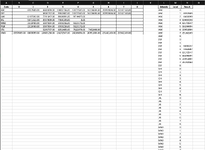
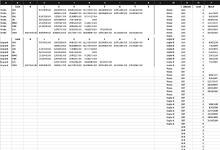
In short, I have a list of the country, jobcode and the level (every eventuality) and then what I expect in column n is for it to concatenate the country, job code and level and then look at the table on the left and pull the value. I think it needs to be index match but I really cannot get my head around it.

Probably very simple to some, but yeah - I cannot do it. Thanks in advance as always!

 

[Fluff]

How about

Fluff.xlsm
	A	B	C	D	E	F	G	H	I	J	K	L	M	N
1		0	1	2	3	4	5	6	7	8
2	A		812	309	727	618	311	134	238	235		A	0
3	B	480	275	147	690		723	227	347	156		A	1	812
4	C	604	699	618	216	926	748	258	811	432		A	2	309
5	D	213	178	291	425	939	379	898	232	867		A	3	727
6	E	737	990	918	744	523	425	695	876	105		A	4	618
7	F	988	633	184	677	503	551	541	486	293		A	5	311
8	G	452	377	303	126	394	775	699	127	861		A	6	134
9	H	457	962	805	560	907	487	187	970	903		A	7	238
10		957		333	673	287	189	102	609			A	8	235
11												B	0	480
12												B	1	275
13												B	2	147
14												B	3	690
15												B	4
16												B	5	723
17												B	6	227
18												B	7	347
19												B	8	156
20												C	0	604
21												C	1	699
22												C	2	618
23												C	3	216
Sheet6

Cell Formulas
Range	Formula
L2:L23	L2	=INDEX($A$2:$A$9,CEILING(ROWS(L$2:L2)/9,1))
M2:M23	M2	=INDEX($B$1:$J$1,,MOD(ROWS(M$2:M2)-1,9)+1)
N2:N23	N2	=IFERROR(1/(1/INDEX($B$2:$J$9,CEILING(ROWS(N$2:N2)/9,1),MOD(ROWS(N$2:N2)-1,9)+1)),"")

 

[nathangwynmorris]

@Fluff! I added an incorrect screenshot - I have one more condition to factor in; country! Sorry if this takes up more of your time!

 

[Fluff]

That is completely different as you now have two different tables & not one.

 

[nathangwynmorris]

Yeah, sorry about that. If it isn't possible then I can just manually change the range for each one and get the results in a different column. But what you did originally did work! And thank you for automating the ABC 0-8 too! That also blew my mind!

 

[Fluff]

Are you still using xl 2013?

 

[nathangwynmorris]

@Fluff I will update that now. I am using the 365 version - v.16.83 on Mac

 

[Fluff]

Thanks for that.
Clear columns M:P & put the formula in M2 only

Fluff.xlsm
	A	B	C	D	E	F	G	H	I	J	K	L	M	N	O	P
1			0	1	2	3	4	5	6	7	8
2	W	A		812	309	727	618	311	134	238	235		W	A	0	0
3	W	B	480	275	147	690		723	227	347	156		W	A	1	812
4	W	C	604	699	618	216	926	748	258	811	432		W	A	2	309
5	W	D	213	178	291	425	939	379	898	232	867		W	A	3	727
6	W	E	737	990	918	744	523	425	695	876	105		W	A	4	618
7	W	F	988	633	184	677	503	551	541	486	293		W	A	5	311
8	W	G	452	377	303	126	394	775	699	127	861		W	A	6	134
9	W	H	457	962	805	560	907	487	187	970	903		W	A	7	238
10													W	A	8	235
11			0	1	2	3	4	5	6	7	8		E	K	0	0
12	E	K		812	309	727	618	311	134	238	235		E	K	1	812
13	E	L	480	275	147	690		723	227	347	156		E	K	2	309
14	E	M	604	699	618	216	926	748	258	811	432		E	K	3	727
15	E	N	213	178	291	425	939	379	898	232	867		E	K	4	618
16	E	O	737	990	918	744	523	425	695	876	105		E	K	5	311
17	E	P	988	633	184	677	503	551	541	486	293		E	K	6	134
18	E	Q	452	377	303	126	394	775	699	127	861		E	K	7	238
19	E	R	1	2	3	4	5	6	7	8	9		E	K	8	235
20													W	B	0	480
21													W	B	1	275
22													W	B	2	147
23													W	B	3	690
24													W	B	4	0
25													W	B	5	723
26													W	B	6	227
27													W	B	7	347
28													W	B	8	156
29													E	L	0	480
30													E	L	1	275
Sheet6

Cell Formulas
Range	Formula
M2:P145	M2	=LET(d,CHOOSEROWS(VSTACK(A2:K9,A12:K19),1,9,2,10,3,11,4,12,5,13,6,14,7,15,8,16),HSTACK(TOCOL(IF(SEQUENCE(,9),INDEX(d,,1))),TOCOL(IF(SEQUENCE(,9),INDEX(d,,2))),TOCOL(IF(SEQUENCE(16),C1:K1)),TOCOL(DROP(d,,2))))
Dynamic array formulas.

 

[nathangwynmorris]

WOWZA! Thanks so much @Fluff. Perfect!

 

[Fluff]

You're welcome & thanks for the feedback.