UK Property Tax SDLT

[DavidHum]

Hi

SDLT

You have featured the UK Property Tax, SDLT, in earlier posts but the Calculations are for a fixed cost of Property.

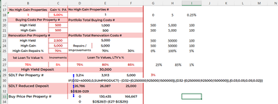
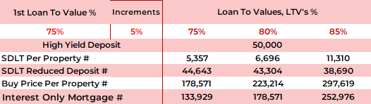
Assuming a Cash Pot of £50,000 and a Mortgage of 75% of Value (LTV), except for the SDLT I could buy a £200,000 Property but I need to withold money to pay the SDLT.

Say the SDLT is 3% of the Buy Price, on £200,000 that is £6,000.

But if I reduce the Cash Pot by £6,000 to £44,000, the maximum Buy Price reduces to £176,000 at 75% LTV with a new SDLT liability at 3% or £5,280.

If the difference of £720 is added to the Deposit, I could increase the Buy Price by up to £2,880, less the increasing SDLT

Without using iteration how can I get an absolutely accurate calc? The code will be in an Online Calculator.

Thankyou David Humphreys

 

[Dave Patton]

It is awkward when the posts relating to one question are on different threads or different areas of the forum'
I made a post and it does not show. With clear and correct information, the posts can be helpful.
The post that follows uses the rates that you cited but this does not agree to your example.
The posts show different results since the brackets and rates are unclear.

To complete the post below,
I renamed the Lambda with #2 to reflect this set of Brackets and Rates.
I edited the formula and provided 2 versions of it.

A few lines of VBA can replicate the formulas to a series of amounts.

T240203a.xlsm
	A	B	C	D	E	F	G	H	I
1								Brackets	Rates
2	Purchase price	182,857.14	200,714.29	218,571.43	147,142.86	111,428.57
3	LTV	75%						0	0%
4	Down Payment	25%						40,000	3%
5	Cash	45,714.29	50,178.57	54,642.86	36,785.71	27,857.14		250,000	8%
6	SDLT	4,285.71	4,821.43	5,357.14	3,214.29	2,142.86		925,000	13%
7	Total cash	50,000.00	55,000.00	60,000.00	40,000.00	30,000.00		1,500,000	15%
8
9	Alternatives
10	SDLT	4,285.71	4,821.43	5,357.14	3,214.29	2,142.86
11		4,285.71	4,821.43	5,357.14	3,214.29	2,142.86
12
1cc

Cell Formulas
Range	Formula
B5:F5	B5	=B2*$B$4
B6:F6	B6	=SDLT_Tax2($H$3:$I$7,B2)
B7:F7	B7	=SUM(B5:B6)
B10:F10	B10	=LET(s,B2,b,{0,40000,250000,925000,1500000},r,{0,0.03,0.05,0.05,0.02},SUM((s>b)*(s-b)*r))
B11	B11	=SUM((B2>$H$3:$H$7)*(B2-$H$3:$H$7)*(I$3:$I$7-$I$2:$I$6))
C11:F11	C11	=SUM((C2>$H$3:$H$7)*(C2-$H$3:$H$7)*($I$3:J$7-$I$2:$I$6))

Lambda Functions
Name	Formula
SDLT_Tax2	=LAMBDA(rngRateData,PurchasePrice,LET(rng,rngRateData,s,PurchasePrice,b,CHOOSECOLS(rng,1),r,CHOOSECOLS(rng,2),ro,VSTACK(0,DROP(r,-1)),SUM((s>b)*(s-b)*(r-ro))))

 

[DavidHum]

Hi Dave

Thank you for the time and effort you have put into this problem of mine, much appreciated, my knowledge of Excel is nowhere near as extensive as yours to the extent that I don’t understand/cannot read your LAMBDA Function even though I have Googled LAMBDA's

I have tried changing row order of your spreadsheet, Purchase Price through Total Cash to the order in my Calculator but can’t make it work.

Also I am confused as there isn't a Formula behind the Purchase Price, B2, or in the Cell Formulas though I can see that B2 features in B6 & B7 but how is it calculated.

Also have tried unsuccessfully to attach my Calculator spreadsheet to a reply but that doesn’t work.

My Cell Order is aimed at taking the User Investor through this section step-by-step to point out how the Cash Deposit is reduced by the amount of the SDLT which is a Variable based on the final Purchase Price.

1st Row, I start with the LTV with 3 options, the User inputs the 1st LTV and the Incremental difference say 5% for the next 2, result 75%, 80% & 85% in 3 columns, the purpose is to be able to compare 3 different Property Values which result in different £ Gross Yields & Capital Gains.

2nd Row, is the single finite amount of Cash that the User has to invest, say £50,000, as the Deposit, which is common across all 3 LTV columns.

3rd Row is the SDLT at the following %’s,

=IF(D32<40000,0,SUMPRODUCT(--(D32>{0;250000;925000;1500000}),(D32-{0;250000;925000;1500000}),{0.03;0.05;0.05;0.02}))

<40,000​	0%​
>39,999 <250,000​	3%​
250,001 - 925,000​	8%​
925,001 - 1.5 M​	13%​
> 1.5 M​	15%​

for each Purchase Price

4th Row is the revised, initially reduced, Deposit on which a new Purchase Price is based for each LTV.

5th Row is the Purchase Price, Reduced/Revised Deposit * LTV Multiple

6th Row, a Mortgage is calculated, Purchase Price * LTV.

This results in a Circular Reference and the only way I know to resolve it is to switch on Iteration which I know is not the answer

This Calculator is one of 25 that breakdown each single element of Buy To Let in the UK but also apply to Property Investment anywhere in the world, even Canada.

The Calculator looks at the high Buying Costs and reduced Asset Values in creating an initial Portfolio of more than 3 Properties which are sufficient for adequate Risk Spread, hence the Variable LTV’s because most Investors will still want positive Cash Flow.

How is life in Calgary? I once passed through in the 60’s travelling by Greyhound from Vancouver to Toronto, almost non-stop and before the trans-highway had been completed so a lot of the timewas spent on gravel!

Again, thankyou for any help you can provide. but please keep it simple if you can.

 

[Dave Patton]

Your questions and comments:
1. "Also I am confused as there isn't a Formula behind the Purchase Price, B2, or in the Cell Formulas though I can see that B2 features in B6 & B7 but how is it calculated."

B2 is the purchase price. The Goal Seek modifies this amount based on the cash amount and the SDLT.

2. " =IF(D32<40000,0,SUMPRODUCT(--(D32>{0;250000;925000;1500000}),(D32-{0;250000;925000;1500000}),{0.03;0.05;0.05;0.02}))"

The brackets and rates are not the same as the information used for the last post.

In the last post, I showed 3 alternatives to the formula.
- which version do you prefer?
Are you using Goal Seek to calculate the purchase price?
If not you may have work with examples starting from the purchase price.


If this works for you and if you want the Lambda formula that requires Excel 365, you can build the Lambda or request another post.

I will provide another example in the next post.
You can copy the post to a clean sheet.
Click on the icon below the f(x) in the Heading, move to your sheet, and select cell A1 and paste.

 

[Dave Patton]

N.B. The Lambda formula requires Excel 365.
To try the Lambda, use Excel's Name Manager
- new type a user friendly name I used SDLT_Tax3
- value copy and paste the Lambda details
(The function shows the required parameters the range with the Brackets and Rates and the Purchase Amount.

T240203a.xlsm
	A	B	C	D	E	F	G	H	I
1								Brackets	Rates
2	Purchase price	182,857.14	200,714.29	218,571.43	35,714.29	39,999.99
3	LTV	75%						0	3%
4	Down Payment	25%						250,000	8%
5	Cash	45,714.29	50,178.57	54,642.86	8,928.57	10,000.00		925,000	13%
6	SDLT	5,485.71	6,021.43	6,557.14	0.00	0.00		1,500,000	15%
7	Total cash	51,200.00	56,200.00	61,200.00	8,928.57	10,000.00
8
9	Alternatives
10	SDLT	5,485.71	6,021.43	6,557.14	0.00	0.00
11	SDLT	5,485.71	6,021.43	6,557.14	0.00	0.00
1cc

Cell Formulas
Range	Formula
B5:F5	B5	=B2*$B$4
B6:F6	B6	=SDLT_Tax3($H$3:$I$6,B2)
B7:F7	B7	=SUM(B5:B6)
B10:F10	B10	=LET(s,B2,b,{0,250000,925000,1500000},r,{0.03,0.05,0.05,0.02},IF(s<40000,0,SUM((s>b)*(s-b)*r)))
B11:F11	B11	=IF(B2<40000,0,SUM((B2>$H$3:$H$6)*(B2-$H$3:$H$6)*($I$3:$I$6-$I$2:$I$5)))

Lambda Functions
Name	Formula
SDLT_Tax3	=LAMBDA(rngRateData,PurchasePrice,LET(rng,rngRateData,s,PurchasePrice,b,CHOOSECOLS(rng,1),r,CHOOSECOLS(rng,2),ro,VSTACK(0,DROP(r,-1)),IF(s<40000,0,SUM((s>b)*(s-b)*(r-ro)))))

 

[DavidHum]

Hi Dave

Unfortunately, I have never used Goal Seek before but have now Googled it to try and find any examples that mimic what I am trying to achieve, that is to initially reduce the Purchase Price Deposit after calculating the SDLT, but nothing come close.

I don’t understand your Spreadsheet, you keep repeating the Total Cash with one LTV when I need 1 Total Cash, 3 Net Cash of SDLT under 3 LTV’s

I have rechecked the SDLT Rates and are as per my last message.

Please can you modify your Spreadsheet as per the attached image from my Calculator covering the relevant Cells, the normal Circular Reference that arises has been sorted by switching on Iteration which of course is just a temporary measure.

Rgds David

 

[DavidHum]

Sorry missed out the attached

 

[Dave Patton]

Good luck with your project.

 

[Dave Patton]

1. Please use correct Brackets and Rates; your formula and rate information in post #12 are different.
2. I used SumProduct for this post.
3. Review the first example and ensure that it is correct.

4. Use Goal Seek
Assume you want to know the Purchase Price with available cash of 60000
Select cell C8
Choose the function Data | What-If-Analysis | Goal Seek
To Value: enter 60000
By Changing: C2
Click OK

T240203a.xlsm
	A	B	C
1
2	Purchase price	170,000.00	178,571.43
3	Loan	75%	75%
4	Down Payment	25%	25%
5	Loan	127,500.00
6	Down Payment	42,500.00	44,642.86
7	SDLT	5,100.00	5,357.14
8	Total cash	47,600.00	50,000.00
1ccc

Cell Formulas
Range	Formula
B5	B5	=B2*B3
B6:C6	B6	=B2*B4
B7:C7	B7	=LET(s,B2,b,{0,250000,925000,1500000},r,{0.03,0.05,0.05,0.02},IF(s<40000,0,SUMPRODUCT(--(s>b),(s-b),r)))
B8	B8	=B6+B7
C8	C8	=SUM(C6:C7)

T240203a.xlsm
	A	B	C	D	E	F	G
1
2	Purchase price	170,000.00	214,285.71	217,391.30	271,739.13	35,714.29	39,999.99
3	Loan	75%	75%	80%	85%	75%	75%
4	Down Payment	25%	25%	20%	15%	25%	25%
5	Loan	127,500.00
6	Down Payment	42,500.00	53,571.43	43,478.26	40,760.87	8,928.57	10,000.00
7	SDLT	5,100.00	6,428.57	6,521.74	9,239.13	0.00	0.00
8	Total cash	47,600.00	60,000.00	50,000.00	50,000.00	8,928.57	10,000.00
1ccc

Cell Formulas
Range	Formula
B5	B5	=B2*B3
B6:E6	B6	=B2*B4
F6:G6	F6	=F2*$C$4
B7:G7	B7	=LET(s,B2,b,{0,250000,925000,1500000},r,{0.03,0.05,0.05,0.02},IF(s<40000,0,SUMPRODUCT(--(s>b),(s-b),r)))
B8	B8	=B6+B7
C8:G8	C8	=SUM(C6:C7)

 

[DavidHum]

First, thankyou for continuing with this post, I thought your Good Luck comment was the end of your help.

Yes, the SDLT Calc in the 1st example is correct.

But, I still can't make your scenarios work and to avoid any typos or differences in the SDLT Rates, I am copying and pasting your Formula into a mirror image spreadsheet, Columns A-C, Rows 2-8, though I don't understand why you are extending to Col G. at max I am only covering 3 Cols for 2-4 Properties?.

Rgds

David

 

[Dave Patton]

"I thought your Good Luck comment was the end of your help." correct.

"Yes, the SDLT Calc in the 1st example is correct." OK

1. copy the example into a clean sheet.
(post 13 You can copy the post to a clean sheet.
Click on the icon below the f(x) in the Heading, move to your sheet, and select cell A1 and paste.)

2. Goal Seek
Assume you want to know the Purchase Price with available cash of 60000
With your computer mouse,
Select (click on) cell C8
move to the menu at the top and click on the the Data group, then the What-If-Analysis subgroup, and then the Goal Seek function
Goal Seek "Set Cell" should show "C8" since you selected that cell
"Value" enter 60000 (we want 60000 per available cash assumption )
"By Changing Cell" enter C2
pause a second and Excel will calculate the result. To accept the result click on OK.

You can then try the process on the other columns and then retry if you want other numbers.
If you do not want column G, delete that column.

T240203a.xlsm
	A	B	C	D	E	F	G	H	I
1								Brackets	Rates
2	Purchase price	170,000.00	214,285.71	217,391.30	271,739.13	39,999.996
3	Loan	75%	75%	80%	85%	75%		0	3%
4	Down Payment	25%	25%	20%	15%	25%		250,000	8%
5	Loan	127,500.00	160,714.29	173,913.04	230,978.26	30,000.00		925,000	13%
6	Down Payment	42,500.00	53,571.43	43,478.26	40,760.87	10,000.00		1,500,000	15%
7	SDLT	5,100.00	6,428.57	6,521.74	9,239.13	0.00
8	Total cash	47,600.00	60,000.00	50,000.00	50,000.00	10,000.00
1ccc

Cell Formulas
Range	Formula
B5:F5	B5	=B2*B3
B6:F6	B6	=B2*B4
B7:F7	B7	=IF(B2<40000,0,SUMPRODUCT(--(B2>$H$3:$H$6),(B2-$H$3:$H$6),($I$3:$I$6-$I$2:$I$5)))
B8	B8	=B6+B7
C8:F8	C8	=SUM(C6:C7)