VBA - find last row and add formula

GeorgeTimes

New Member
Joined
Jul 22, 2022
Messages
16
Office Version
  1. 365
  2. 2021
  3. 2019
  4. 2016
  5. 2013
  6. 2011
  7. 2010
  8. 2007
Platform
  1. Windows
Hi all,

I need your help for a VBA code that does the next:

Find first blank cell in column A (I have this) : Range("A" & Rows.Count).End(xlUp).Offset(1).Select

Once you found the last column from A, I need to populate this formula till last row based on column G : =G4. So I will have:

A10 has value =G10
A13 has value =G13 and so on...


My issue is:

1 - If last row in G column is 50, and the first empty row in column A is 40, then I need a code to paste the formula to A40 - A50. I'm not sure how to write that code in order to paste within this range (the range will be different every time I run the code)

2 - how can I modify the formula from =G4 to =G40, =G41 etc. if I don't know what row will be the last one when I run the macro. The number of row needs to be the same in column A and column G. Again, I'm not sure how I can change the number from the formula as next time I run the code I can start from row 70 for example


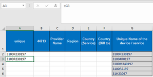
I've attached an example of this. A2 and A3 already have the formula, G6 is the last row so I need a vba to fill in from A4 till A6 the next:
A4: =G4
A5: =G5
A6: =G6
 

Attachments

  • Capture.PNG
    Capture.PNG
    14 KB · Views: 24

Excel Facts

Create a chart in one keystroke
Select the data and press Alt+F1 to insert a default chart. You can change the default chart to any chart type
Hi,

does this do what you need ?
VBA Code:
Sub add_formula()

Dim x, Alastrow, Glastrow As Long

Alastrow = ActiveSheet.Cells(Rows.Count, 1).End(xlUp).Row 'use col 1 for bottom
Glastrow = ActiveSheet.Cells(Rows.Count, 7).End(xlUp).Row 'use col 7 for bottom


For x = Alastrow To Glastrow

ActiveSheet.Range("A" & x).Value = "=G" & x

Next x


End Sub
 
Upvote 0
Hi and welcome to MrExcel board!

Try this:

VBA Code:
Sub PutFormula()
  Range("A4:A" & Range("G" & Rows.Count).End(3).Row).Formula = "=G4"
End Sub
 
Upvote 0
Hi and welcome to MrExcel board!

Try this:

VBA Code:
Sub PutFormula()
  Range("A4:A" & Range("G" & Rows.Count).End(3).Row).Formula = "=G4"
End Sub
Thanks for your reply.

I forgot to mention, but I need something that will not add the formula to the rest of column A. In A2 and A3, there will be values, not formula, the macro will add the formula to A4,A5 etc, then I will copy paste them as values. I need it this way as my data has +10k rows and it gets bigger every month. I also need to have formulas in multiple columns and that's why I'm trying to avoid adding a formula to all the rows as it will take quite some time for Excel to calculate this.
 
Upvote 0
ok, try this one
VBA Code:
Sub add_formula()

Dim x, Alastrow, Glastrow As Long

Alastrow = ActiveSheet.Cells(Rows.Count, 1).End(xlUp).Row 'use col 1 for bottom
Glastrow = ActiveSheet.Cells(Rows.Count, 7).End(xlUp).Row 'use col 1 for bottom


For x = Alastrow To Glastrow

    ActiveSheet.Range("A" & x).Value = ActiveSheet.Range("G" & x).Value

Next x


End Sub
 
Upvote 0
Hi,

does this do what you need ?
VBA Code:
Sub add_formula()

Dim x, Alastrow, Glastrow As Long

Alastrow = ActiveSheet.Cells(Rows.Count, 1).End(xlUp).Row 'use col 1 for bottom
Glastrow = ActiveSheet.Cells(Rows.Count, 7).End(xlUp).Row 'use col 7 for bottom


For x = Alastrow To Glastrow

ActiveSheet.Range("A" & x).Value = "=G" & x

Next x


End Sub
Hi Rob,

Thanks for this, it works, however with one small error - if A3 is first blank cell, it start to add the formula from A2. However, I've managed to fix this by adding Offset(1) to Alastrow.

If I'm not asking for too much, are you able to help me with the below formula as well? I need the same thing, find what row number needs to be added, however the formula is an XLOOKUP.

=XLOOKUP(I7,Sheet1!G3:G10,Sheet1!J3:J10,"")

Everything remains the same, i.e G is the longest column, I need to locate first blank row for I column and then add the XLOOKUP formula till last row (G column). But again, I don't know which one is the first blank row in I, so I need a way to amend I7 to the relevant row number.

Tried the below but it doesn't work: ActiveSheet.Range("A" & x).Value = "=XLOOKUP("=G" & x,Sheet1!G3:G10,Sheet1!J3:J10,"""")"
 
Upvote 0
ah, yes, sorry I saw that but forgot to correct it. Simply add a "+1" in the line as follows: that way it starts from the next blank, rather than the last row. I guess it doesn't affect your results as the data is the same anyway ?

VBA Code:
For x = Alastrow + 1 To Glastrow

    ActiveSheet.Range("A" & x).Value = ActiveSheet.Range("G" & x).Value

Next x

which column is this Xlookup formula being added to - is it A again ?
The data is the same in this example, I've tried to give you an easy example I use for column A, however I use more "complicated formulas" in other columns and I thought based on your answer I can figure things out for the other columns. Turns out I can't :)

Yes, you can add the Xlookup formula in column A (I can manage to amend that afterwards as I have different Xlookup in other columns and I'll take your example in order to amend those)
 
Upvote 0
Hi George,
sorry - re-reading your posts, I can't catch what your formula is doing. You have a value in I7 that you want to lookup in G3:g10, and output that in J3:10 ??
Then you speak about not knowing what is lastrow in Col I ..

I'm a little confused sorry - please be specific with columns you are using, and what you are trying to look up please ?
thanks
Rob
 
Upvote 0
See if this works for you.

Typically you would do the replace around the whole formula string
Actually might need to rethink the below since the LastRowG is now of the lookup table in a different sheet but I have to go.

VBA Code:
Sub FillDownFormulaXlookup()
    '=XLOOKUP(I7,Sheet1!G3:G10,Sheet1!J3:J10,"")
    Dim shtMain As Worksheet
    Dim rng As Range
    Dim lastRowA As Long, lastRowG As Long
   
    Set shtMain = ActiveSheet
   
    With shtMain
        lastRowA = .Range("A" & Rows.Count).End(xlUp).Row
        lastRowG = Worksheets("Sheet1").Range("G" & Rows.Count).End(xlUp).Row
        Set rng = .Range(.Cells(lastRowA + 1, "A"), .Cells(lastRowG, "A"))
        rng.Formula = "=XLookup($I" & lastRowA + 1 & Replace(",Sheet1!$G$3:$G$#,Sheet1!$J$3:$J$#,"""")", "#", lastRowG)
        rng.Value = rng.Value
    End With
   
End Sub
 
Last edited:
Upvote 0

Forum statistics

Threads
1,215,280
Messages
6,124,034
Members
449,139
Latest member
sramesh1024

We've detected that you are using an adblocker.

We have a great community of people providing Excel help here, but the hosting costs are enormous. You can help keep this site running by allowing ads on MrExcel.com.
Allow Ads at MrExcel

Which adblocker are you using?

Disable AdBlock

Follow these easy steps to disable AdBlock

1)Click on the icon in the browser’s toolbar.
2)Click on the icon in the browser’s toolbar.
2)Click on the "Pause on this site" option.
Go back

Disable AdBlock Plus

Follow these easy steps to disable AdBlock Plus

1)Click on the icon in the browser’s toolbar.
2)Click on the toggle to disable it for "mrexcel.com".
Go back

Disable uBlock Origin

Follow these easy steps to disable uBlock Origin

1)Click on the icon in the browser’s toolbar.
2)Click on the "Power" button.
3)Click on the "Refresh" button.
Go back

Disable uBlock

Follow these easy steps to disable uBlock

1)Click on the icon in the browser’s toolbar.
2)Click on the "Power" button.
3)Click on the "Refresh" button.
Go back
Back
Top