VBA PivotTable with Conditional Formatting Speed Issue

[bl4met]

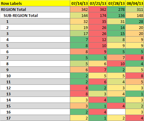
I have been struggling with this for a while now. What I have works but is slow. I have a pivot table that I am generating in VBA on command and then I use the code below to run a conditional format. my problem is that I need row to have each number only compared to the others in the same row not the whole table. So at this point I am looping through the whole table. The problem is that the table can be a few thousand rows long and it taking forever and excel stops responding from time to time. And I'm doing this on 2 different sheets to boot.

This is my loop. It has to be able to grow with the table length and width wise as one table is a set number of columns but the other table's number of columns increase hourly.

Do Until Range("A" & r).Value = "Grand Total"
    With Range(Cells(r, 2), Cells(r, i))
        .FormatConditions.AddColorScale ColorScaleType:=3
        With .FormatConditions(1)
            With .ColorScaleCriteria(1)
                .Type = xlConditionValueLowestValue
                With .FormatColor
                    .Color = 8109667
                    .TintAndShade = 0
                End With
            End With
            With .ColorScaleCriteria(2)
                .Type = xlConditionValuePercentile
                .Value = 50
                With .FormatColor
                    .Color = 8711167
                    .TintAndShade = 0
                End With
            End With
            With .ColorScaleCriteria(3)
                .Type = xlConditionValueHighestValue
                With .FormatColor
                    .Color = 7039480
                    .TintAndShade = 0
                End With
            End With
        End With
    End With
    r = r + 1
Loop

I'm writing this in xl2010 but need it to work in xl2007. Any help would be appreciated. I've been self teaching myself this via google for the most part.

 

[Fazza]

hi,

from a quick glance, you're looping through a lot of rows applying the conditional formatting row by row

instead can the conditionall formatting be applied to the entire range in one operation, without looping?

I only work in Excel 2003 so can not test the particular conditional format used

basically the first line & two last lines of code would be removed - the "do until" & the "r=r+1" and "loop"

and the new first instead of With Range(cells(r,2),cells(r,i))
changes to suit the pivot table range

there are various ways to refer to the pivot table range, the pivot table has some ranges, the object browswer can help identify them. or just as easy maybe is .find "Grand Total" and use from the top of the pivot table to the row above the grand total. so you might end up with "With range(cells(first row, 2),cells(row above grand total, i))" or something like that

hth

 

[bl4met]

That would work except that I want each row compared to itself. The rows of the table are regions and the columns are weeks and I'm trying to compare the current week to the 4 previous weeks for each region. each region is also further broken down so if i did say pt.databodyrange except that would compare in the column as well as the row. For the data ranges in a pivot table, the best for me would probably be pt.pivotfields.pivotitems.datarange but I would still need to loop through that with 4 nested for each loops.

 

[Fazza]

That would work except that I want each row compared to itself.

How is that a problem? It is routine for conditional formatting - in Excel 2003 & earlier anyway. Using relative cell references can handle this. So a simple conditional format formula applied to the entire range: and no looping.

An image would help.

It sounds like you want to compare a column with the four columns on its left. If the cell is the minimum give it one color or the maximum give it a different color.

If that isn't what you're doing, would it be OK?

regards

PS. Can you create the conditional formatting you want in one step for the entire range of one pivot table? Maybe it is just the VBA that is the hurdle.

 

[bl4met]

I haven't found a way to do what I am looking for manually other than going line by line and that usually just applying the formatting to the first line and using the format painter to copy to the next one and so on. Below is an image of a sample table with the desired output. I'm comparing totals for the day to the totals for the previous 4 weeks on the same day. I need to know this not only by region but sub region and users. Right now the table when fully expanded is 1500 rows but as the day goes on i expect it to hit around 3000 rows.

 

[Fazza]

OK, thanks.

I'm in Excel 2003 which has limited conditional formatting compared to later versions. One can have only three conditions - plus a base colour to allow four colours. This is close to what you want & I'm sure you can adjust it for Excel 2007.

I'm on holidays for a while after today, btw. so may not respond til next month

hth

'this demonstrates the idea - syntax details may be different in your Excel version
'I've assumed the fields to be formatted are in columns C:F, adjust as required

with range("your range to be formatted")

  .formatconditions.delete

  .formatconditions.add type:=xlexpression, formula1:="=rc=max(rc3:rc6)"
  .formatconditions(1).interior.colorindex = 3

  .formatconditions.add type:=xlexpression, formula1:="=rc=min(rc3:rc6)"
  .formatconditions(2).interior.colorindex = 50

  .formatconditions.add type:=xlexpression, formula1:="=rc=large(rc3:rc6,2)"
  .formatconditions(3).interior.colorindex = 45

  .interior.colorindex = 43

end with

 

[bl4met]

That worked thank you. I ended up with

With pt.DataBodyRange


    .FormatConditions.Delete
    
    .FormatConditions.Add Type:=xlExpression, Formula1:="=rc=max(rc2:rc6)"
    .FormatConditions(1).Interior.Color = RGB(255, 77, 51)
    
    .FormatConditions.Add Type:=xlExpression, Formula1:="=rc=min(rc2:rc6)"
    .FormatConditions(2).Interior.Color = RGB(61, 245, 0)
    
    .Interior.Color = RGB(255, 255, 122)


End With

I may have have to change it if the powers that be don't like it but i have having issues finding colors that I liked for each level of value.