vba to find the sum product of filtered data

[abhi_jain80]

Hi,

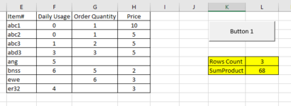
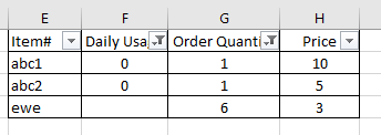
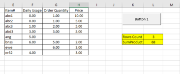
I have filtered the data using the below vba code which is filtering the rows if column G is not blank and column F is 0 and column F is blank.

Range("L6") = Application.CountIfs(Columns("G:G"), "<>", Columns("F:F"), "=0") + Application.CountIfs(Columns("G:G"), "<>", Columns("F:F"), "")

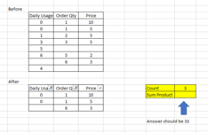
The count of rows filtered out is 3 which is fine. Now I need to find the sum product of column G and column H of the filtered data but struggling to get the code, can somebody help me please? Image attached...

Apologies if this has been solved earlier and thanks in advance...

Abhi

 

[Domenic]

The following code assumes that the worksheet containing the data is the active worksheet, uses Column H to determine the last row, and places the result in M6...

    Dim lastRow As Long
    lastRow = Cells(Rows.Count, "H").End(xlUp).Row
   
    With Range("A10")
        .Formula = "=SUMPRODUCT(SUBTOTAL(3,OFFSET(G2:G" & lastRow & ",ROW(G2:G" & lastRow & ")-ROW(G2),0,1)),G2:G" & lastRow & ",H2:H" & lastRow & ")"
        .Value = .Value
    End With

Hope this helps!

 

[abhi_jain80]

The following code assumes that the worksheet containing the data is the active worksheet, uses Column H to determine the last row, and places the result in M6...

    Dim lastRow As Long
    lastRow = Cells(Rows.Count, "H").End(xlUp).Row
   
    With Range("A10")
        .Formula = "=SUMPRODUCT(--SUBTOTAL(3,OFFSET(G2:G" & lastRow & ",ROW(G2:G" & lastRow & ")-ROW(G2),0,1)),G2:G" & lastRow & ",H2:H" & lastRow & ")"
        .Value = .Value
    End With

Hope this helps!

Hi Domenic,

Thanks for replying. It is giving me the sum product of all the values but not of the filtered rows appeared in Range("L6"). It seems like I am missing something. Based on the sample data, I am getting 68 as an answer while it should be 33. Here is the code I am using:

Sub Button1_Click()
Range("L6") = Application.CountIfs(Columns("G:G"), "<>", Columns("F:F"), "=0") + Application.CountIfs(Columns("G:G"), "<>", Columns("F:F"), "")

Dim lastRow As Long
lastRow = Cells(Rows.Count, "E").End(xlUp).Row
With Range("L7")
.Formula = "=SUMPRODUCT(--SUBTOTAL(3,OFFSET(G2:G" & lastRow & ",ROW(G2:G" & lastRow & ")-ROW(G2),0,1)),G2:G" & lastRow & ",H2:H" & lastRow & ")"
.Value = .Value
End With
End Sub

 

[Domenic]

It looks like your data is not filtered, and the formula is correctly returning 68 for the displayed data. Or am I missing something?

By the way, I amended my formula to remove the double negative ( -- ), which isn't needed for the calculation. So the resulting value doesn't change.

 

[abhi_jain80]

It looks like your data is not filtered, and the formula is correctly returning 68 for the displayed data. Or am I missing something?

By the way, I amended my formula to remove the double negative ( -- ), which isn't needed for the calculation. So the resulting value doesn't change.

Currently the formula is returning 68 but I want it to return 33. Actually, I need the sum product of only 3 rows (as attached in the image) which got filtered by applying the condition as column G is not blank and column F is 0 and column F is blank.

Hope I am clear now with the requirement. Thanks.

 

[Domenic]

The formula is correct, and as such should return 33, unless the numbers in your data are being recognized as text values instead of numerical values. Does this return the correct result?

        .Formula = "=SUMPRODUCT(SUBTOTAL(3,OFFSET(G2:G" & lastRow & ",ROW(G2:G" & lastRow & ")-ROW(G2),0,1)),G2:G" & lastRow & "+0,H2:H" & lastRow & "+0)"

 

[abhi_jain80]

The formula is correct, and as such should return 33, unless the numbers in your data are being recognized as text values instead of numerical values. Does this return the correct result?

        .Formula = "=SUMPRODUCT(SUBTOTAL(3,OFFSET(G2:G" & lastRow & ",ROW(G2:G" & lastRow & ")-ROW(G2),0,1)),G2:G" & lastRow & "+0,H2:H" & lastRow & "+0)"

Apologies...I have converted all the values to numeric and updated the formula as you said but still getting the same answer 68 not 33.

 

[Domenic]

I don't know how you converted those values into numeric values, so it's possible that they may still be recognized as text values. Can you please try the last formula I posted, and tell us the result?

 

[abhi_jain80]

I don't know how you converted those values into numeric values, so it's possible that they may still be recognized as text values. Can you please try the last formula I posted, and tell us the result?

I have formatted all the cells to number. Is this not the right way? My result is still 68. This is the code I am using now:

Sub Button1_Click()
Range("L6") = Application.CountIfs(Columns("G:G"), "<>", Columns("F:F"), "=0") + Application.CountIfs(Columns("G:G"), "<>", Columns("F:F"), "")

Dim lastRow As Long
lastRow = Cells(Rows.Count, "E").End(xlUp).Row
With Range("L7")
.Formula = "=SUMPRODUCT(SUBTOTAL(3,OFFSET(G2:G" & lastRow & ",ROW(G2:G" & lastRow & ")-ROW(G2),0,1)),G2:G" & lastRow & "+0,H2:H" & lastRow & "+0)"
.Value = .Value
End With
End Sub

 

[Domenic]

Sorry, I see that you had already tried my last formula, which means that they were already being correctly recognized as numerical values.

So the formula should return the desired result based on the filtered data.