VLOOKUP and match return in whole column

YellowTangerine

New Member
Joined
Mar 5, 2023
Messages
29
Office Version
  1. 365
Platform
  1. Windows
  2. MacOS
Hello, I'm new here. Apologies ahead of I don't use the correct terminology.

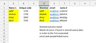
I have data coming from two sources that I need to combine and match on a spreadsheet. The answers can't be returned in a single cell but match through and answered for each row in a column.

One source supplies just a name in one column and a unique code for each name in a second column.

The second source supplies the name (which matches the first source) but also an email address and another name associated with the name in the first source.

I need to bring all three pieces of information together into one worksheet and wondered if there is a way to use the VLOOKUP to populate cell in a column with a match, rather than just returning an answer in one cell.

Thank you in advance for your support.
 

Excel Facts

Ambidextrous Undo
Undo last command with Ctrl+Z or Alt+Backspace. If you use the Undo icon in the QAT, open the drop-down arrow to undo up to 100 steps.
Can you provide some sample source, sample destination and some desired result?
 
Upvote 0
Here's an example of raw data from one system in the left. On the right is the desire outcome. Source data from second source includes name, address, email etc but not included. I'm am a basic spreadsheet user. Hope this helps. Thank you in advance.
 

Attachments

  • IMG_20230305_090050_665.jpg
    IMG_20230305_090050_665.jpg
    64.4 KB · Views: 14
Upvote 0
Here's an example of raw data from one system in the left. On the right is the desire outcome. Source data from second source includes name, address, email etc but not included. I'm am a basic spreadsheet user. Hope this helps. Thank you in advance.
I forgot to say, I must have the unique ID remain with the first name. I will be doing a mailmerge and the unique ID will go into the body of the letter. It's used to set up an account for Name 1.
 
Upvote 0
This is a simple VLOOKUP issue. I don't get what you mean by "match the whole column". You can automate it with getting index from column:
Excel Formula:
=VLOOKUP($A2,$H$2:$J$5,COLUMN(A1),0)

1678008220042.png
 
Upvote 0
This is a simple VLOOKUP issue. I don't get what you mean by "match the whole column". You can automate it with getting index from column:
Excel Formula:
=VLOOKUP($A2,$H$2:$J$5,COLUMN(A1),0)

View attachment 86786
Thank you. I'll go and see if I can replicate this. Sorry about my poor terminology. I need to match all the data so that each Name 1 column is correctly matched to the correct email address in the second source data. Hope that makes better sense?
 
Upvote 0
Thank you. I'll go and see if I can replicate this. Sorry about my poor terminology. I need to match all the data so that each Name 1 column is correctly matched to the correct email address in the second source data. Hope that makes better sense?
What does getting from index column mean?
 
Upvote 0
Thank you. I'll go and see if I can replicate this. Sorry about my poor terminology. I need to match all the data so that each Name 1 column is correctly matched to the correct email address in the second source data. Hope that makes better sense?
I now understand. Thank you. How can I ensure the Unique ID is included in the result of the VLOOKUP please?
 
Upvote 0
This is a simple VLOOKUP issue. I don't get what you mean by "match the whole column". You can automate it with getting index from column:
Excel Formula:
=VLOOKUP($A2,$H$2:$J$5,COLUMN(A1),0)

View attachment 86786
Thank you so much. I am uploading a sample data spreadsheet which should make it much clearer. This is a new area for me. I'm so grateful for your support. I hope you will be able to see the outcome I now desire and my apologies for the poor communication from my side. Please see below:

POC Data 050323.xlsx
ABCDEFGHIJKLM
1Child NameUnique CodeChild Name Unique CodeParent NameParent EmailParent NameParent EmaiChild Name
2Child 3359fh4#N/A#N/A#N/AName 1test1@gmail.comChild 1
3Child 1359fh5#N/A#N/A#N/AName 2test2@gmail.comChild 2
4Child 5359fh6#N/A#N/A#N/AName 3test3@gmail.comChild 3
5Child 4359fh7#N/A#N/A#N/AName 4test4@gmail.comChild 4
6Child 2359fh8#N/A#N/A#N/AName 5test5@gmail.comChild 5
7Child 6359fh9#N/A#N/A#N/AName 6test6@gmail.comChild 6
8
9Data Source 1ResultData Source 2
Sheet1
Cell Formulas
RangeFormula
E2:E7,G2:G7E2=VLOOKUP($A2:$A7,$K$2:$M$7,COLUMN(A1),0)
F2:F7F2=VLOOKUP($B2:$B7,COLUMN(B1),0)
Dynamic array formulas.
 
Upvote 0

Forum statistics

Threads
1,215,558
Messages
6,125,504
Members
449,235
Latest member
Terra0013

We've detected that you are using an adblocker.

We have a great community of people providing Excel help here, but the hosting costs are enormous. You can help keep this site running by allowing ads on MrExcel.com.
Allow Ads at MrExcel

Which adblocker are you using?

Disable AdBlock

Follow these easy steps to disable AdBlock

1)Click on the icon in the browser’s toolbar.
2)Click on the icon in the browser’s toolbar.
2)Click on the "Pause on this site" option.
Go back

Disable AdBlock Plus

Follow these easy steps to disable AdBlock Plus

1)Click on the icon in the browser’s toolbar.
2)Click on the toggle to disable it for "mrexcel.com".
Go back

Disable uBlock Origin

Follow these easy steps to disable uBlock Origin

1)Click on the icon in the browser’s toolbar.
2)Click on the "Power" button.
3)Click on the "Refresh" button.
Go back

Disable uBlock

Follow these easy steps to disable uBlock

1)Click on the icon in the browser’s toolbar.
2)Click on the "Power" button.
3)Click on the "Refresh" button.
Go back
Back
Top