vlookup dictionary approximate match

roykana

Active Member
Joined
Mar 8, 2018
Messages
311
Office Version
  1. 2010
Platform
  1. Windows
Dear all Master,
below I want the desired result in column E which I marked in yellow and also I use a formula so it's easy to understand what I mean and I want to add a little in the code below without changing the structure of the code below and I also made a vba code for in column E in sheet "selectfile" with marking red but it doesn't work because I'm also wrong in the code
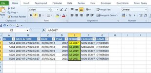
VBA Code:
Sub vloookupdictionary()
Dim Rng As Range, Ds As Range, n As Long, Dic As Object, Source As Variant
Dim Ary As Variant
Dim startTime As Double
Dim endTime As Double
Dim t
t = Timer
endTime = Timer
'Dim startTime As Double
'Dim endTime As Double
Application.ScreenUpdating = False
[COLOR=rgb(209, 72, 65)]With Sheets("DB")
    Source = .Range("C1").CurrentRegion.Resize(, 4)
End With
Set Dic = CreateObject("scripting.dictionary")
Dic.CompareMode = vbBinaryCompare
For n = 2 To UBound(Source, 1)
    Dic(Source(n, 1)) = n
Next

[COLOR=rgb(209, 72, 65)]'result in column E Sheet "selectfile"
With Sheets("SELECTFILE")
    Ary = .Range("C2", .Range("C" & Rows.Count).End(xlUp)).Value2
    ReDim Nary(1 To UBound(Ary), 1 To 3)
    For n = 1 To UBound(Ary)
        If Dic.Exists(Ary(n, 1)) Then
            Nary(n, 1) = Source(Dic(Ary(n, 1)), 4)
        End If
    Next n
    .Range("E2").Resize(UBound(Nary), 1).Value = Nary
End With
With Sheets("DB")
    Source = .Range("i1").CurrentRegion.Resize(, 4)
End With[/COLOR]
Set Dic = CreateObject("scripting.dictionary")
Dic.CompareMode = vbTextCompare
For n = 2 To UBound(Source, 1)
    Dic(Source(n, 1)) = n
Next[/COLOR]
With Sheets("SELECTFILE")
    Ary = .Range("A2", .Range("A" & Rows.Count).End(xlUp)).Value2
    ReDim Nary(1 To UBound(Ary), 1 To 3)
    For n = 1 To UBound(Ary)
        If Dic.Exists(Ary(n, 1)) Then
            Nary(n, 1) = Source(Dic(Ary(n, 1)), 3)
            Nary(n, 2) = Source(Dic(Ary(n, 1)), 2)
        End If
    Next n
    .Range("F2").Resize(UBound(Nary), 2).Value = Nary
End With


Application.ScreenUpdating = True

'Debug.Print "Demo-03????:" & amp; amp; endTime - startTime
Debug.Print "It's done in: " & Timer - t & " seconds"
Debug.Print "Time to complete = " & Timer - startTime & " seconds."
End Sub


desired result
Book3
ABCDEFG
1IDDATE & TIMEDATEYEARPERIODCATEGORYNAME
250142017-07-27 07:42:2327/07/20172017Jul-2017NON STAFFOTHERS01
350042018-07-27 07:43:3127/07/20182018Jul-2018MANAGEROTHERS02
450162017-07-27 07:45:2327/07/20192019Jul-2019NON STAFFOTHERS03
550202017-07-27 07:46:2627/07/20202020Jul-2020NON STAFFOTHERS04
650082017-07-27 07:48:1727/07/20212021Jul-2021NON STAFFOTHERS04
SELECTFILE
Cell Formulas
RangeFormula
E2:E6E2=VLOOKUP(C2,Table1,4,1)


source table
vlookup dictionary approximate match.xlsm
CDEFGHIJKL
1DATE1DATE2PERIOD1PERIOD2IDNAMECATEGORYLOCATION
221/07/201720/07/201701 Juli-2017Jul-20175014OTHERS01NON STAFFSHOP01
327/07/201820/07/201801 Juli-2018Jul-20185004OTHERS02MANAGERSHOP02
427/07/201920/07/201901 Juli-2019Jul-20195016OTHERS03NON STAFFSHOP03
527/07/202020/07/202001 Juli-2020Jul-20205020OTHERS04NON STAFFSHOP04
627/07/202120/07/202101 Juli-2021Jul-20215008OTHERS04NON STAFFSHOP05
DB


Thanks
roykana
 
Last edited:
According to your post #5 attachment I would take the obvious easy path :​
VBA Code:
Sub Demo0()
    With Sheet1.Range("E2:E" & Sheet1.UsedRange.Rows.Count)
        .Formula = "=VLOOKUP(C2,Table1,4,1)"
        .Formula = .Value
    End With
End Sub
But according to your post #9 where you need column E as text​
- this information was not in the initial post (as it must be !) where the picture is showing dates instead of texts ! Is is so difficult to just well explain your need ? -​
this is the revamped version :​
VBA Code:
Sub Demo1()
        Dim V, R&
        Application.ScreenUpdating = False
    With Sheet1.Range("E2:E" & Sheet1.UsedRange.Rows.Count)
       .Formula = "=VLOOKUP(C2,Table1,4,1)"
        V = .Value
        For R = 1 To UBound(V):  V(R, 1) = CStr(V(R, 1)):  Next
       .NumberFormat = "@"
       .Value2 = V
    End With
        Application.ScreenUpdating = True
End Sub
@Marc L

thank you for your reply, if I do it with xlbb as below, then copy it to excel, then the format will be a date but the original format is general in column E and you can also see in the screenshot below which shows the format is general


vlookup dictionary approximate match.xlsm
E
1PERIOD
2Jul-2017
3Jul-2018
4Jul-2019
5Jul-2020
6Jul-2021
SELECTFILE
 

Attachments

  • Capture29012022.JPG
    Capture29012022.JPG
    73.8 KB · Views: 9
Upvote 0

Excel Facts

How to create a cell-sized chart?
Tiny charts, called Sparklines, were added to Excel 2010. Look for Sparklines on the Insert tab.
The reason why it's better in some case to link a workbook with a crystal clear & complete explanation in the first post …​
 
Upvote 0
@Marc L
can the format be general if it is text then the result is as below?


IMPORT FILE DAT DB ABSEN V.3.xlsm
ABCDEFG
1IDDATE & TIMEDATEYEARPERIODCATEGORYNAME
250142017-07-27 07:42:2327/07/20172017=IFERROR(VLOOKUP(C2,dbperiod,4,1),"")NON STAFFBAYU
350042017-07-27 07:43:3127/07/20172017=IFERROR(VLOOKUP(C2,dbperiod,4,1),"")STAFFAJENG KARTINI
450162017-07-27 07:45:2327/07/20172017=IFERROR(VLOOKUP(C2,dbperiod,4,1),"")NON STAFFRAHMAN
550202017-07-27 07:46:2627/07/20172017=IFERROR(VLOOKUP(C2,dbperiod,4,1),"")NON STAFFYOSEP
650082017-07-27 07:48:1727/07/20172017=IFERROR(VLOOKUP(C2,dbperiod,4,1),"")STAFFADE SUPRIATNA
SELECTFILE
 
Upvote 0
@shknbk2

thanks for your reply. I tried it was appropriate but the result should be text or general in column E in the "selectfile" sheet because the source is not a date format so I have to add code like below or do you have other recommendations

VBA Code:
.Columns(5).NumberFormat = "@"
For my code, I would use your suggestion and put it right above the Value assignment for E2:
VBA Code:
        .Columns(5).NumberFormat = "@"
        .Range("E2").Resize(UBound(Nary), 3).Value = Nary

In the download of your file, I notice that you had apostrophes in Col F of DB. Are those in the raw data of a normal spreadsheet or did you have to put them in the example data to make them text?
 
Upvote 0
For my code, I would use your suggestion and put it right above the Value assignment for E2:
VBA Code:
        .Columns(5).NumberFormat = "@"
        .Range("E2").Resize(UBound(Nary), 3).Value = Nary

In the download of your file, I notice that you had apostrophes in Col F of DB. Are those in the raw data of a normal spreadsheet or did you have to put them in the example data to make them text

@shknbk2


Yes, that's raw data from a normal spreadsheet
 
Upvote 0
The reason why it's better in some case to link a workbook with a crystal clear & complete explanation in the first post …​
@Marc L
I have a recent post for you related to dat files

 
Upvote 0

Precision about my previous post : when a VBA procedure allocates a formula to a cell the cell must not be formatted as text …​
 
Upvote 0
Precision about my previous post : when a VBA procedure allocates a formula to a cell the cell must not be formatted as text …​
@Marc L

yes, you are right, so before the vba formula procedure, the column was already in clear format
 
Upvote 0

Forum statistics

Threads
1,214,979
Messages
6,122,559
Members
449,089
Latest member
Motoracer88

We've detected that you are using an adblocker.

We have a great community of people providing Excel help here, but the hosting costs are enormous. You can help keep this site running by allowing ads on MrExcel.com.
Allow Ads at MrExcel

Which adblocker are you using?

Disable AdBlock

Follow these easy steps to disable AdBlock

1)Click on the icon in the browser’s toolbar.
2)Click on the icon in the browser’s toolbar.
2)Click on the "Pause on this site" option.
Go back

Disable AdBlock Plus

Follow these easy steps to disable AdBlock Plus

1)Click on the icon in the browser’s toolbar.
2)Click on the toggle to disable it for "mrexcel.com".
Go back

Disable uBlock Origin

Follow these easy steps to disable uBlock Origin

1)Click on the icon in the browser’s toolbar.
2)Click on the "Power" button.
3)Click on the "Refresh" button.
Go back

Disable uBlock

Follow these easy steps to disable uBlock

1)Click on the icon in the browser’s toolbar.
2)Click on the "Power" button.
3)Click on the "Refresh" button.
Go back
Back
Top