vlookup with match to return a result with multiple rows with lookup value

[excelnoob_67]

So I have a doozy of a question.

I have 2 tables.
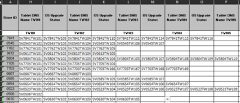
Table 1: contains a list "Sites=siteID" on each row. Columns contain "Device Name" 1-30
Table 2: contains "SiteID", "Device Name" SiteID is over multiple rows

See examples
Table 1:

Site ID	Device Name 001	Device Name 002	Device Name 003
7412	LAP7412001	LAP7412002	LAP7412003
9632	LAP9632001	LAP9632002	LAP9632003

Table 2:

7412	LAP7412001
7412	LAP7412002
7412	LAP7412003
9632	LAP9632001
9632	LAP9632002
9632	LAP9632003

Now what I would like to do is match / vlookup the data in table 2 and update table 1 column Device Name.
In my head it would be something like:
lookup 7412 if device name = 7412001 add it column 001
lookup 7412 if device name = 7412002 add it column 002
And so on and so on.

first issue is vlookup wont look past the first siteID on table 2. Table is not a large export and can be formatting another way to make is easier to look up.
I guess the real question is how can I tell excel if the siteid matches and the device id ends in 001/2/3 add to the relevant columns

This isn't a simple transpose will fix situation

Any help would be appreciate

Thanks

 

[FormR]

Hi, how about something like this:

Book1
	A	B	C	D
1	Site ID	Device Name 001	Device Name 002	Device Name 003
2	7412	LAP7412001	LAP7412002	LAP7412003
3	9632	LAP9632001	LAP9632002	LAP9632003
4	9999	LAP9632001	LAP9632002
5
6	Table 2:
7	7412	LAP7412001
8	7412	LAP7412002
9	7412	LAP7412003
10	9632	LAP9632001
11	9632	LAP9632002
12	9632	LAP9632003
13	9999	LAP9632002
14	9999	LAP9632001
Sheet1

Cell Formulas
Range	Formula
B4:C4,B2:D3	B2	=TRANSPOSE(SORT(FILTER($B$7:$B$14,$A$7:$A$14=A2)))
Dynamic array formulas.

 

[excelnoob_67]

Hi, how about something like this:

Book1
	A	B	C	D
1	Site ID	Device Name 001	Device Name 002	Device Name 003
2	7412	LAP7412001	LAP7412002	LAP7412003
3	9632	LAP9632001	LAP9632002	LAP9632003
4	9999	LAP9632001	LAP9632002
5
6	Table 2:
7	7412	LAP7412001
8	7412	LAP7412002
9	7412	LAP7412003
10	9632	LAP9632001
11	9632	LAP9632002
12	9632	LAP9632003
13	9999	LAP9632002
14	9999	LAP9632001
Sheet1

Cell Formulas
Range	Formula
B4:C4,B2:D3	B2	=TRANSPOSE(SORT(FILTER($B$7:$B$14,$A$7:$A$14=A2)))
Dynamic array formulas.

Hi FormR

Really close!
Thats returns the correct result and in numerical order but doesnt match up with my headers. It also automatically spills over in to the next cells

See screenshot
ignore row 2 I was seeing if I could match it as an unique ID

 

[FormR]

See screenshot

Hi, can you repost the new sample data and layout using same method you did in the first post - so we can copy and paste it to Excel, rather than re-type it.

 

[excelnoob_67]

Hi, can you repost the new sample data and layout using same method you did in the first post - so we can copy and paste it to Excel, rather than re-type it.

I'm just walking out of the door of the office ill post it once I get home. Thanks.

 

[FormR]

You could also consider exploring XL2BB as way to show your sample data and layout.

XL2BB - Excel Range to BBCode

Excel 'mini-sheet' in messages - XL2BB Although experts prefer to read your description and question instead of working in your actual file to solve your problem, there are times that it is difficult to explain an issue without providing actual...

www.mrexcel.com

 

[excelnoob_67]

This is the full data set below.
Hopefully this makes some more sense

TIA

Table 1:

Store ID	Tablet DNS Name TW101	OS Upgrade Status	Tablet DNS Name TW102	OS Upgrade Status	Tablet DNS Name TW103	OS Upgrade Status	Tablet DNS Name TW104	OS Upgrade Status	Tablet DNS Name TW105	OS Upgrade Status	Tablet DNS Name TW106
	TW101		TW102		TW103		TW104		TW105		TW106
7841
0545
7762
0613
5804
7705
7703
0667
0585
0654
0523
0506
0630

Table 2:

Store ID	System Name
0506	SV0506TW102
0523	SV0523TW101
0523	SV0523TW102
0523	SV0523TW103
0523	SV0523TW104
0523	SV0523TW105
0523	SV0523TW106
0523	SV0523TW107
0523	SV0523TW108
0523	SV0523TW109
0545	SV0545TW102
0545	SV0545TW103
0545	SV0545TW104
0545	SV0545TW105
0545	SV0545TW106
0545	SV0545TW107
0585	SV0585TW102
0585	SV0585TW103
0585	SV0585TW104
0585	SV0585TW105
0585	SV0585TW106
0585	SV0585TW107
0613	SV0613TW101
0613	SV0613TW102
0613	SV0613TW104
0613	SV0613TW105
0630	SV0630TW101
0630	SV0630TW102
0630	SV0630TW103
0630	SV0630TW104
0630	SV0630TW105
0654	SV0654TW101
0654	SV0654TW102
0654	SV0654TW103
0654	SV0654TW104
0654	SV0654TW105
0654	SV0654TW106
0654	SV0654TW107
0667	SV0667TW101
0667	SV0667TW102
0667	SV0667TW103
5804	SV5804TW101
5804	SV5804TW102
5804	SV5804TW103
5804	SV5804TW104
5804	SV5804TW105
5804	SV5804TW107
5804	SV5804TW108
5804	SV5804TW109
5804	SV5804TW110
7703	SV7703TW102
7703	SV7703TW103
7703	SV7703TW105
7703	SV7703TW166
7703	SV7703TW167
7703	SV7703TW168
7703	SV7703TW169
7705	SV7705TW101
7705	SV7705TW102
7705	SV7705TW103
7705	SV7705TW104
7762	SV7762TW101
7762	SV7762TW103
7762	SV7762TW104
7762	SV7762TW105
7841	SV7841TW101
7841	SV7841TW103
7841	SV7841TW104
7841	SV7841TW110
7841	SV7841TW111
7841	SV7841TW114
7841	SV7841TW115
7841	SV7841TW116

 

[FormR]

Hi, if I've understood correctly, you could try this copied down and across.

Book3
	A	B	C	D	E	F	G	H	I	J	K	L
1	Store ID	Tablet DNS Name TW101	OS Upgrade Status	Tablet DNS Name TW102	OS Upgrade Status	Tablet DNS Name TW103	OS Upgrade Status	Tablet DNS Name TW104	OS Upgrade Status	Tablet DNS Name TW105	OS Upgrade Status	Tablet DNS Name TW106
2		TW101		TW102		TW103		TW104		TW105		TW106
3	7841	SV7841TW101				SV7841TW103		SV7841TW104
4	545			SV0545TW102		SV0545TW103		SV0545TW104		SV0545TW105		SV0545TW106
5	7762	SV7762TW101				SV7762TW103		SV7762TW104		SV7762TW105
6	613	SV0613TW101		SV0613TW102				SV0613TW104		SV0613TW105
7	5804	SV5804TW101		SV5804TW102		SV5804TW103		SV5804TW104		SV5804TW105
8	7705	SV7705TW101		SV7705TW102		SV7705TW103		SV7705TW104
9	7703			SV7703TW102		SV7703TW103				SV7703TW105
10	667	SV0667TW101		SV0667TW102		SV0667TW103
11	585			SV0585TW102		SV0585TW103		SV0585TW104		SV0585TW105		SV0585TW106
12	654	SV0654TW101		SV0654TW102		SV0654TW103		SV0654TW104		SV0654TW105		SV0654TW106
13	523	SV0523TW101		SV0523TW102		SV0523TW103		SV0523TW104		SV0523TW105		SV0523TW106
14	506			SV0506TW102
15	630	SV0630TW101		SV0630TW102		SV0630TW103		SV0630TW104		SV0630TW105
16
17	Table 2:
18	Store ID	System Name
19	506	SV0506TW102
20	523	SV0523TW101
21	523	SV0523TW102
22	523	SV0523TW103
23	523	SV0523TW104
24	523	SV0523TW105
25	523	SV0523TW106
26	523	SV0523TW107
27	523	SV0523TW108
28	523	SV0523TW109
29	545	SV0545TW102
30	545	SV0545TW103
31	545	SV0545TW104
32	545	SV0545TW105
33	545	SV0545TW106
34	545	SV0545TW107
35	585	SV0585TW102
36	585	SV0585TW103
37	585	SV0585TW104
38	585	SV0585TW105
39	585	SV0585TW106
40	585	SV0585TW107
41	613	SV0613TW101
42	613	SV0613TW102
43	613	SV0613TW104
44	613	SV0613TW105
45	630	SV0630TW101
46	630	SV0630TW102
47	630	SV0630TW103
48	630	SV0630TW104
49	630	SV0630TW105
50	654	SV0654TW101
51	654	SV0654TW102
52	654	SV0654TW103
53	654	SV0654TW104
54	654	SV0654TW105
55	654	SV0654TW106
56	654	SV0654TW107
57	667	SV0667TW101
58	667	SV0667TW102
59	667	SV0667TW103
60	5804	SV5804TW101
61	5804	SV5804TW102
62	5804	SV5804TW103
63	5804	SV5804TW104
64	5804	SV5804TW105
65	5804	SV5804TW107
66	5804	SV5804TW108
67	5804	SV5804TW109
68	5804	SV5804TW110
69	7703	SV7703TW102
70	7703	SV7703TW103
71	7703	SV7703TW105
72	7703	SV7703TW166
73	7703	SV7703TW167
74	7703	SV7703TW168
75	7703	SV7703TW169
76	7705	SV7705TW101
77	7705	SV7705TW102
78	7705	SV7705TW103
79	7705	SV7705TW104
80	7762	SV7762TW101
81	7762	SV7762TW103
82	7762	SV7762TW104
83	7762	SV7762TW105
84	7841	SV7841TW101
85	7841	SV7841TW103
86	7841	SV7841TW104
87	7841	SV7841TW110
88	7841	SV7841TW111
89	7841	SV7841TW114
90	7841	SV7841TW115
91	7841	SV7841TW116
Sheet1

Cell Formulas
Range	Formula
B3:L15	B3	=IF(B$2="","",INDEX(FILTER($B$19:$B$91,($A$19:$A$91=$A3)*(RIGHT($B$19:$B$91,LEN(B$2))=B$2),""),1))

 

[excelnoob_67]

Hi, if I've understood correctly, you could try this copied down and across.

Book3
	A	B	C	D	E	F	G	H	I	J	K	L
1	Store ID	Tablet DNS Name TW101	OS Upgrade Status	Tablet DNS Name TW102	OS Upgrade Status	Tablet DNS Name TW103	OS Upgrade Status	Tablet DNS Name TW104	OS Upgrade Status	Tablet DNS Name TW105	OS Upgrade Status	Tablet DNS Name TW106
2		TW101		TW102		TW103		TW104		TW105		TW106
3	7841	SV7841TW101				SV7841TW103		SV7841TW104
4	545			SV0545TW102		SV0545TW103		SV0545TW104		SV0545TW105		SV0545TW106
5	7762	SV7762TW101				SV7762TW103		SV7762TW104		SV7762TW105
6	613	SV0613TW101		SV0613TW102				SV0613TW104		SV0613TW105
7	5804	SV5804TW101		SV5804TW102		SV5804TW103		SV5804TW104		SV5804TW105
8	7705	SV7705TW101		SV7705TW102		SV7705TW103		SV7705TW104
9	7703			SV7703TW102		SV7703TW103				SV7703TW105
10	667	SV0667TW101		SV0667TW102		SV0667TW103
11	585			SV0585TW102		SV0585TW103		SV0585TW104		SV0585TW105		SV0585TW106
12	654	SV0654TW101		SV0654TW102		SV0654TW103		SV0654TW104		SV0654TW105		SV0654TW106
13	523	SV0523TW101		SV0523TW102		SV0523TW103		SV0523TW104		SV0523TW105		SV0523TW106
14	506			SV0506TW102
15	630	SV0630TW101		SV0630TW102		SV0630TW103		SV0630TW104		SV0630TW105
16
17	Table 2:
18	Store ID	System Name
19	506	SV0506TW102
20	523	SV0523TW101
21	523	SV0523TW102
22	523	SV0523TW103
23	523	SV0523TW104
24	523	SV0523TW105
25	523	SV0523TW106
26	523	SV0523TW107
27	523	SV0523TW108
28	523	SV0523TW109
29	545	SV0545TW102
30	545	SV0545TW103
31	545	SV0545TW104
32	545	SV0545TW105
33	545	SV0545TW106
34	545	SV0545TW107
35	585	SV0585TW102
36	585	SV0585TW103
37	585	SV0585TW104
38	585	SV0585TW105
39	585	SV0585TW106
40	585	SV0585TW107
41	613	SV0613TW101
42	613	SV0613TW102
43	613	SV0613TW104
44	613	SV0613TW105
45	630	SV0630TW101
46	630	SV0630TW102
47	630	SV0630TW103
48	630	SV0630TW104
49	630	SV0630TW105
50	654	SV0654TW101
51	654	SV0654TW102
52	654	SV0654TW103
53	654	SV0654TW104
54	654	SV0654TW105
55	654	SV0654TW106
56	654	SV0654TW107
57	667	SV0667TW101
58	667	SV0667TW102
59	667	SV0667TW103
60	5804	SV5804TW101
61	5804	SV5804TW102
62	5804	SV5804TW103
63	5804	SV5804TW104
64	5804	SV5804TW105
65	5804	SV5804TW107
66	5804	SV5804TW108
67	5804	SV5804TW109
68	5804	SV5804TW110
69	7703	SV7703TW102
70	7703	SV7703TW103
71	7703	SV7703TW105
72	7703	SV7703TW166
73	7703	SV7703TW167
74	7703	SV7703TW168
75	7703	SV7703TW169
76	7705	SV7705TW101
77	7705	SV7705TW102
78	7705	SV7705TW103
79	7705	SV7705TW104
80	7762	SV7762TW101
81	7762	SV7762TW103
82	7762	SV7762TW104
83	7762	SV7762TW105
84	7841	SV7841TW101
85	7841	SV7841TW103
86	7841	SV7841TW104
87	7841	SV7841TW110
88	7841	SV7841TW111
89	7841	SV7841TW114
90	7841	SV7841TW115
91	7841	SV7841TW116
Sheet1

Cell Formulas
Range	Formula
B3:L15	B3	=IF(B$2="","",INDEX(FILTER($B$19:$B$91,($A$19:$A$91=$A3)*(RIGHT($B$19:$B$91,LEN(B$2))=B$2),""),1))

Worked great Thanks!

final formula below for my specific sheet
=IF(H$2="","",INDEX(FILTER('[Copy of Book1.xlsx]Sheet1'!$B$2:$B$74,('[Copy of Book1.xlsx]Sheet1'!$A$2:$A$74=$A3)*(RIGHT('[Copy of Book1.xlsx]Sheet1'!$B$2:$B$74,LEN(H$2))=H$2),""),1))

 

[excelnoob_67]

@FormR as my excel start to go the processing time for al the formulas is becoming really slow. can we adjust the formula to lookup the first say 1200 rows opposed to the entire column?