VLOOKUP With Same Values

[Selects]

As you can see, I'm attempting to show differences between these companies based on these particular values. The problem is many of the companies have the same values, and VLOOKUP just repeats the company with the first value it finds. I'm trying to figure out how to have VLOOKUP realize that there are other companies with the same value, so each company is accounted for.

Thanks,
Selects

 

[Selects]

Bump.

 

[Matty]

Welcome to MrExcel!

I'm not clear what you're trying to do here. Could explain further?

It also doesn't help much when pictures are posted, as we can't copy the data out to test possible solutions in Excel. Try the Excel Jeanie for posting data in future:

http://www.excel-jeanie-html.de/index.php?f=1

Matty

 

[Selects]

Thanks for the warm welcome!

I'm at work and need admin access to install programs, so unfortunately I can't install the excel genie until I can get someone in IT up here.

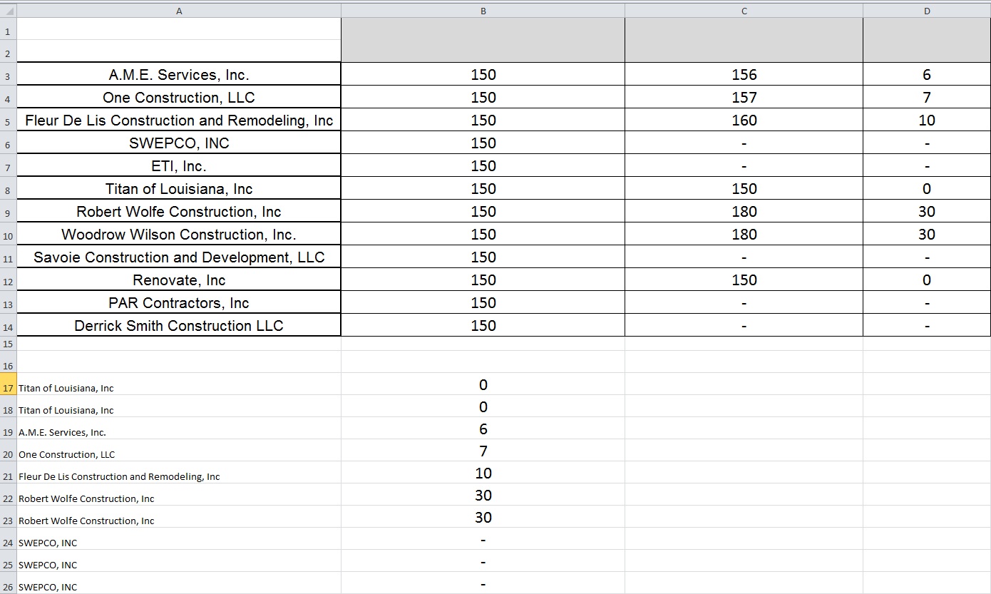
What I am doing is ranking these companies from from least to greatest based on the value in column D. I used the SMALL formula to put the numbers in order from least to greatest in column B (lines 17-26), then used VLOOKUP to relate those numbers back to the company.

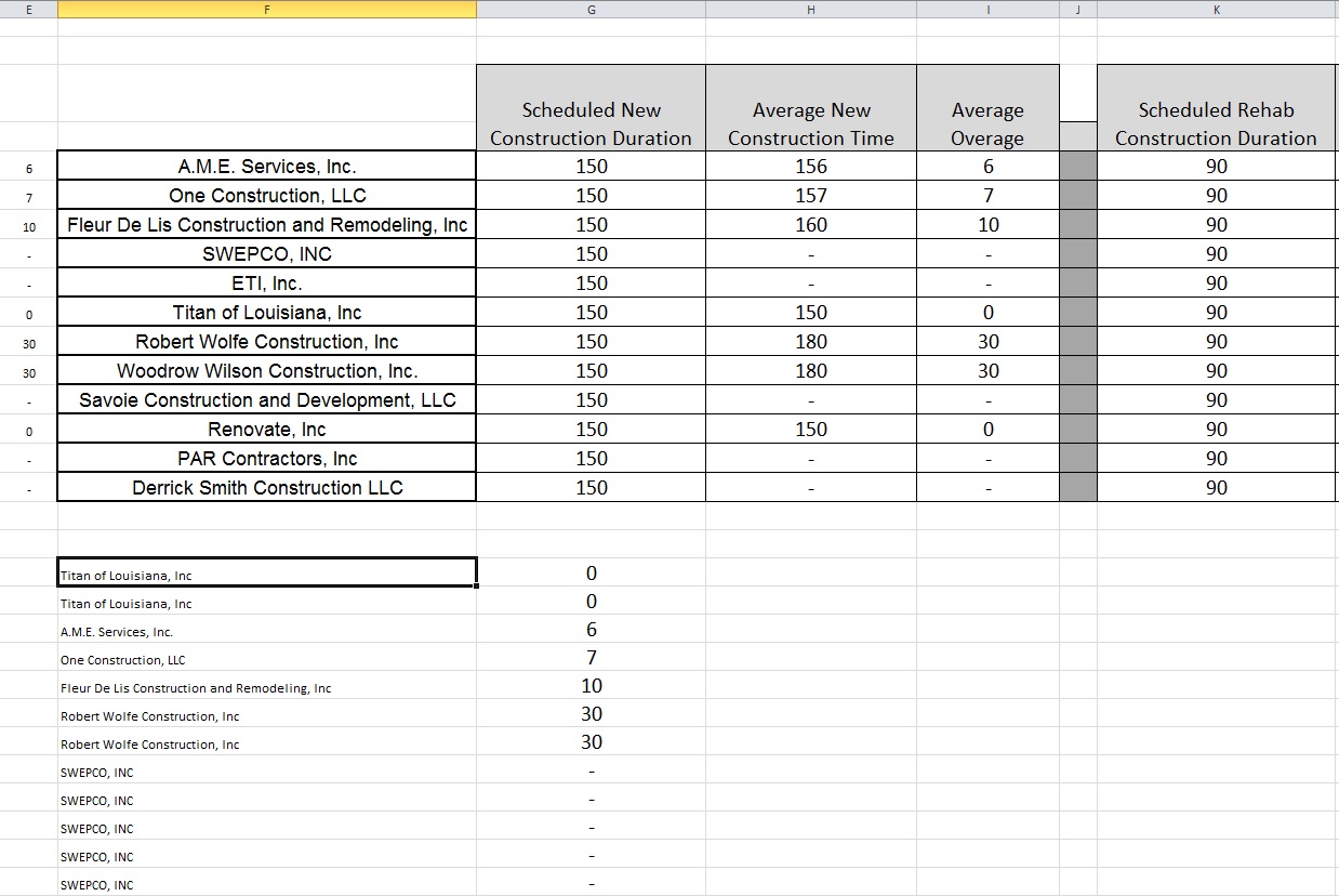
This image should help more:

So the code for A17:A26 looks like this: =VLOOKUP(G23,$E$9:$F$20,2,FALSE)

The values for column "E" are the same as column "I", it's just more convenient to have them next to the companies code-wise.

The problem is that when VLOOKUP pulls the information from column "E", it can't differentiate between the first instance of "0" versus the second instance of "0", and the same goes for the other duplicate amounts. Instead, it always chooses the first value and the corresponding company. So, when the table below should read:
Titan of Louisiana Inc. 0

as the first line, the next line should read:

Renovate, Inc. 0

but, it continues to reference Titan instead.

So, I need to find a way to have each company accounted for, even if the values are the same.

I hope this isn't too confusing.

- Selects

 

[Matty]

See if you can adapt the following suggestion by Aladin:

http://www.mrexcel.com/forum/showthread.php?t=342541

Post #7.

Respond back if you have any issues.

Matty