Want to use VLOOKUP and IF for a code from another workbook

[dudeinaghillie]

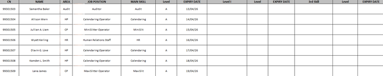
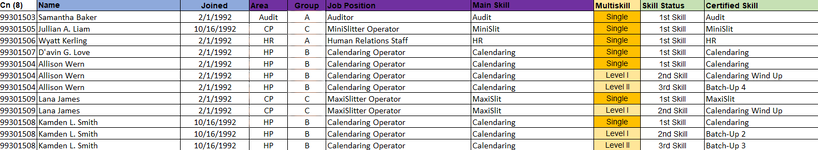
So I have 2 workbooks, the first workbook contains a unique ID in a column as well as columns with name, age, skill level, skill name, expiry date in accordance to the unique ID. **NOTE: 1 Unique IDs may have 1 or more skill levels and skill names, different skill level = different row, same unique ID**
Now in the 2nd workbook, I would like to pull the data of the skill name with relation to the skill level using the unique ID as the input.

This is what I have made and the result is "SPILL!"

IF(VLOOKUP(@A:A,'[Data_Skill.xlsx]Sheet1'!$A$2:$D$5000,4,FALSE)="Level I",(VLOOKUP(@A:A,'[Data_Skill.xlsx]Sheet1'!$E$2:$E$5000,5,FALSE),"No Skill")

A Column being the unique ID and D being skill level and E being skill name.
Would like to know if there is another way of doing this or if anyone can help fix any wrongs in the formula.
If anymore information is needed, please feel free to ask.

Thank you

 

[dudeinaghillie]

Here is another format that I tried but to no avail

=IF(@'[Data_Skill.xlsx]Sheet1'!$D$2:$D$5000="Level I",VLOOKUP(@A:A,'[Data_Skill.xlsx]Sheet1'!$A$2:$L$5000,12,FALSE)," ")

 

[Alex Blakenburg]

Your initial formula has a number of issues.
Firstly, I would not have thought you could get a SPILL error without having MS365 or Excel 2021. (I only have 365 so I can't test to confirm)
Are you really using 2019 ?

Without having dynamic array functionality I would expect the formula to look more like this:
With the formula being on row 2 and then copied down to the other rows

=IF(VLOOKUP(A2,'[Data_Skill.xlsx]Sheet1'!$A$2:$D$5000,4,FALSE)="Level I",VLOOKUP(A2,'[Data_Skill.xlsx]Sheet1'!$A$2:$E$5000,5,FALSE),"No Skill")

 

[dudeinaghillie]

=IF(VLOOKUP(A2,'[Data_Skill.xlsx]Sheet1'!$A$2:$D$5000,4,FALSE)="Level I",VLOOKUP(A2,'[Data_Skill.xlsx]Sheet1'!$A$2:$E$5000,5,FALSE),"No Skill")

Thank you for this reply, I might've changed a few things before copying and pasting in the first part of the post and yes it included errors instead of spill.
Though the formula you provided does not have an error to it, I would like it to return the value_if_true value instead of the value_if_false value, is there a way in doing so.

Thank you again

 

[Alex Blakenburg]

You will need to show me a couple of examples. At the moment if it finds Level I in column D it will return the value in Column E.
Note: I have copied and pasted your text and Level I is using the letter i, it would seem to me that the number 1 is more likely. Is that perhaps the issue you are having ?

 

[dudeinaghillie]

You will need to show me a couple of examples. At the moment if it finds Level I in column D it will return the value in Column E.
Note: I have copied and pasted your text and Level I is using the letter i, it would seem to me that the number 1 is more likely. Is that perhaps the issue you are having ?

Yes, I am using roman numeric, here are the tables, the questions I've asked are altered, but the gist of the column information that I included should hopefully suffice without breaching any privacy of others, if not please tell.

Thank you again for the reply

 

[Alex Blakenburg]

1) if you are going to use pictures you need to show the row and column references and provide the sheet names.
2) Where is the formula going ?
3) what is the expected result ?

 

[dudeinaghillie]

1) if you are going to use pictures you need to show the row and column references and provide the sheet names.
2) Where is the formula going ?
3) what is the expected result ?

Sorry for this late reply,

The formula is supposed to go on the column "Level I" in the first picture.
The expected result is to be "Level I"'s Certified Skill name from the second picture and so forth for Level II, Level III, etc.
What I wanted to do is to pull data using the "Cn" which is the unique ID to show the skill names for different Levels thus the formula would look like this in the first picture's column "Level I":-

=IF(@'[Data_Skill.xlsx]Sheet1'!$H$2:$H$5000="Level I",VLOOKUP(@A:A,'[Data_Skill.xlsx]Sheet1'!$A$2:$J$5000,10,FALSE)," ")

However, the formula above would only display the value_if_false output, instead, what I need from the formula is the value_if_true, corresponding to the Skill Level, in this case Level I, to whatever the Certified Skill for that level is.

Thank you again

 

[Alex Blakenburg]

See if this works for you.

=IFERROR(LOOKUP(2,1/(([Data_Skill.xlsx]Sheet1!$A$2:$A$5000=$A3)*([Data_Skill.xlsx]Sheet1!$H$2:$H$5000=H$1)),[Data_Skill.xlsx]Sheet1!$J$2:$J$5000),"")

 

[dudeinaghillie]

See if this works for you.

=IFERROR(LOOKUP(2,1/(([Data_Skill.xlsx]Sheet1!$A$2:$A$5000=$A3)*([Data_Skill.xlsx]Sheet1!$H$2:$H$5000=H$1)),[Data_Skill.xlsx]Sheet1!$J$2:$J$5000),"")

Thank you so much, this worked well and displayed what I needed, I do have a question as to the part of the code that you provided. What is the 2,1 for?

=IFERROR(LOOKUP(2,1