xlookup, vlookup, hlookup with and/if multiple criteria. Which do I use?

shina67 · Nov 27, 2023

Hi All,

I have a problem with the below which I am hoping one of you genius people can help with.

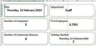
From image 1 the cell B2 is dynamic to any day of the year. Cell F2 is also a drop down which has 16 catergories.

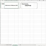
I need to be able to lookup in image 2 based on the 2 above criteria. As you can see in image 1 it clearly says that on 15th Feb there are 2 members of staff on holiday.
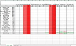
What I need is from image 2 to find out who them 2 members of Staff are.

If the date and Department changed it would need to find if anyone is on holiday from that department and on that date.

Is there a formula that would do this without the need of vba?

I am trying to build this dashboard and planner without the use of vba to try and broaden my formula knowledge.

I have come across some new formula that I haven't used before whilst building this but have come stuck on this part.

I hope what i am trying to achieve is explained properly. Any questions or help would be greatly recieved.

Thanks in advance.

BrerRabbit · Nov 27, 2023

You need an extra column to deal with the dynamic needs of each day.

Simply, put in an extra column, which you can hide if you wish, to show this formula: C22 = =IF(HLOOKUP($C$19,$F$21:$G$24,ROW(A1)+1,FALSE)="H",HLOOKUP($C$19,$F$21:$G$24,ROW(A1)+1,FALSE),IF(HLOOKUP($C$19,$F$21:$G$24,ROW(A1)+1,FALSE)="UA",HLOOKUP($C$19,$F$21:$G$24,ROW(A1)+1,FALSE),""))
where C19 = today().

Instead of "H" and "UA" have them each in a cell and refer to that cell if you wish. Then do a count and whatever math you need in that cell.

If you want to take this one step further and do a report each day of who is on leave and who has UA on that day you can do a match, index offset in a separate location that will list those on holiday.

17

B

C

D

E

F

G

H

I

J

K

L

M

18

find this->

H

19

28-11-23

employees on holiday today

20

match

index

21

Today?

27-11-23

28-11-23

22

zak ellis

UA

H

UA

3

andrew wood

23

andrew wood

H

UA

H

4

ayden windle

24

ayden windle

H

C19 = today()
C21 = =IF(HLOOKUP($C$19,$F$21:$G$24,ROW(A1)+1,FALSE)="H",HLOOKUP($C$19,$F$21:$G$24,ROW(A1)+1,FALSE),IF(HLOOKUP($C$19,$F$21:$G$24,ROW(A1)+1,FALSE)="UA",HLOOKUP($C$19,$F$21:$G$24,ROW(A1)+1,FALSE),""))
K22 =MATCH($L$18,OFFSET($C$21,K21,,1000),0)+K21
L22 =INDEX($B$21:$B$24,K22)

shina67 · Nov 28, 2023

BrerRabbit said:
You need an extra column to deal with the dynamic needs of each day.

Simply, put in an extra column, which you can hide if you wish, to show this formula: C22 = =IF(HLOOKUP($C$19,$F$21:$G$24,ROW(A1)+1,FALSE)="H",HLOOKUP($C$19,$F$21:$G$24,ROW(A1)+1,FALSE),IF(HLOOKUP($C$19,$F$21:$G$24,ROW(A1)+1,FALSE)="UA",HLOOKUP($C$19,$F$21:$G$24,ROW(A1)+1,FALSE),""))
where C19 = today().

Instead of "H" and "UA" have them each in a cell and refer to that cell if you wish. Then do a count and whatever math you need in that cell.

If you want to take this one step further and do a report each day of who is on leave and who has UA on that day you can do a match, index offset in a separate location that will list those on holiday.

17
B C D E F G H I J K L M
18
find this-> H
19
28-11-23
employees on holiday today
20
match index
21
Today?
27-11-23
28-11-23
22
zak ellis UA H UA
3
andrew wood
23
andrew wood H UA H
4
ayden windle
24
ayden windle H H

C19 = today()
C21 = =IF(HLOOKUP($C$19,$F$21:$G$24,ROW(A1)+1,FALSE)="H",HLOOKUP($C$19,$F$21:$G$24,ROW(A1)+1,FALSE),IF(HLOOKUP($C$19,$F$21:$G$24,ROW(A1)+1,FALSE)="UA",HLOOKUP($C$19,$F$21:$G$24,ROW(A1)+1,FALSE),""))
K22 =MATCH($L$18,OFFSET($C$21,K21,,1000),0)+K21
L22 =INDEX($B$21:$B$24,K22)

Hi BrerRabbit,

Thanks for your reply.

When using the formula above and adapted for my sheets and cells I get #N/A returned.
I have adapted the above formula to be :-

=IF(HLOOKUP(Dashboard!$B$2,'Holiday Tracker'!$L$3:$NM$4,ROW(A1)+1,FALSE)="H",HLOOKUP(Dashboard!$B$2,'Holiday Tracker'!$L$7:$NM$999,ROW(A1)+1,FALSE),IF(HLOOKUP(Dashboard!$B$2,'Holiday Tracker'!$L$7:$NM$999,ROW(A1)+1,FALSE)="HH",HLOOKUP(Dashboard!$B$2,'Holiday Tracker'!$L$7:$NM$999,ROW(A1)+1,FALSE),""))

Also on the above formula's where does K21 refer to.

After getting a full list of who is on H or UA I could then use the FILTER formula to just display the Department of who is on H or UA.

I look forward to your reply.

BrerRabbit · Nov 28, 2023

#n/a is bcuz there's no data to be retrieved. Use this:

=IF(HLOOKUP(Dashboard!$B$2,'Holiday Tracker'!$L$3:$NM$4,ROW(A1)+1,FALSE)="H",HLOOKUP(Dashboard!$B$2,'Holiday Tracker'!$L$7:$NM$999,ROW(A1)+1,FALSE),IF(HLOOKUP(Dashboard!$B$2,'Holiday Tracker'!$L$7:$NM$999,ROW(A1)+1,FALSE)="HH",HLOOKUP(Dashboard!$B$2,'Holiday Tracker'!$L$7:$NM$999,ROW(A1)+1,FALSE),""))

Instead of the match, go with filter as you correctly suggested, and try this:

17

B

C

D

E

F

G

H

I

J

K

L

M

18

find this->

H

Dept

blue

19

Dept

28-11-23

employees on holiday today from Dept blue

20

21

Today?

27-11-23

28-11-23

ayden windle

blue

H

22

zak ellis

blue

UA

H

UA

23

andrew wood

Green

H

UA

H

24

ayden windle

blue

H

L3 = =FILTER(B22:D24,($C$22:$C$24=$O$18)*($D$22:$D$24=$M$18),"") giving both the dept and the absence type you requested.

shina67 · Nov 28, 2023

Hi BrerRabbit,

I am probably missing something so very simple but it has been a long couple of days. I cannot seem to get the above to work for me or I have not explained properly.

I have attached a couple more screenshots to hopefully explain a bit better.

So on the 'Dashboard' sheet (dashboard image attached) I am wanting to use the data in cells $B$2 & $F$2 as my criteria.

In the 'Holiday Tracker' sheet (Holiday Tracker image attached) I want to lookup the date from Dashboard!$B$2 & the department from Dashboard!$F$2 and return who is on Holiday.

So the returned values from the attached images should be Martin Leveridge & Paul Ian Hewitt.
If the date in Dashboard!$B$2 was changed to 13th February the returned values should be Kyle Young & Martin Leveridge.

If the department in Dashboard!$F$2 was changed to 'Bifolds' or any of the other 15 departments then the values returned from the attached images would be blank.

Hopefully I can adapt the formula then so I can see who is on Holiday (H or HH), who is on Sick (S & SS) & Unauthorised Absence (UA).

shina67 · Nov 28, 2023

Book1.xlsx

A

B

C

D

E

F

G

H

I

AC

AD

1

2

Wednesday, 14 February 2024

Cut/Prep

3

4

5

6

7

8

9

Dashboard

Book1.xlsx

A

B

AQ

AR

AS

AT

AU

AV

AW

AX

AY

AZ

BA

BB

BC

BD

BE

BF

BG

1

2

3

4

01/02/2024

02/02/2024

03/02/2024

04/02/2024

05/02/2024

06/02/2024

07/02/2024

08/02/2024

09/02/2024

10/02/2024

11/02/2024

12/02/2024

13/02/2024

14/02/2024

15/02/2024

16/02/2024

5

Name

Area

6

7

ASHLEY BAIRSTOW

Adeco

8

HERSCHEL LAKE

Adeco

9

PAUL CUNNINGHAM

Adeco

10

ADAM FLETCHER

Bifolds

11

BRANDON ROBERTSON

Bifolds

12

CHRISTOPHER PEARSON

Bifolds

13

DANIEL JENNINGS

Bifolds

14

DECLAN MILBURN

Bifolds

15

DECLAN MCLAUGHLIN

Bifolds

16

GARY MADDOX

Bifolds

17

GEOFFREY NEIL GREENWOOD

Bifolds

18

JAMIE MILLS

Bifolds

19

JAMIE SHAW

Bifolds

20

JOHN MARTIN FISHER

Bifolds

21

JOHN MORRELL

Bifolds

22

JOSHUA PICKERING

Bifolds

23

LOUIE WHITE

Bifolds

24

MARIA NOEMI DE FREIT JOAO

Bifolds

25

MARK CLEGG

Bifolds

26

MARTIN JOHN WALKER

Bifolds

27

NEIL LORIMER

Bifolds

28

ROBERT MOUNTAIN

Bifolds

29

THEMBA DLAMINI

Bifolds

30

JEAN WILLIAMS

Cleaner

31

KODUA TWENEBOA

Cleaner

32

RUTH AMOAKO

Cleaner

33

SARAH BILTON

Cleaner

34

ALAN PHILIP VICKERS

Cut/Prep

35

ALEX ALHASSAN

Cut/Prep

36

CALLUM SMITH

Cut/Prep

37

DANIEL BRIGHAM

Cut/Prep

38

DARREN JOSEPH SANDERS

Cut/Prep

39

HARRY POWELL

Cut/Prep

40

JOHN COPLAND MCDONALD

Cut/Prep

41

JOHN DAVID MASSINGHAM

Cut/Prep

42

JONATHON PAUL COWLING

Cut/Prep

43

KEITH SMITH

Cut/Prep

44

KYLE YOUNG

Cut/Prep

H

UA

45

MARTIN LEVERIDGE

Cut/Prep

H

46

PAUL IAN HEWITT

Cut/Prep

S

HH

47

48

49

Holiday Tracker

Cell Formulas
Range	Formula
AQ5:BF5	AQ5	=AQ4
AQ6:BF6	AQ6	=TEXT(AQ4,"DDD")

Cells with Conditional Formatting
Cell	Condition		Cell Format	Stop If True
L7:BF46	Cell Value	="L"	text	NO
L7:BF46	Cell Value	="UA"	text	NO
L7:BF46	Cell Value	="SS"	text	NO
L7:BF46	Cell Value	="S"	text	NO
L7:BF46	Cell Value	>0	text	NO
L7:BF46	Cell Value	="HH"	text	NO
L7:BF46	Cell Value	="H"	text	NO
L7:BF46,L5:BF5,L6:AO6,AQ6:BF6	Expression	=L$6="Sun"	text	NO
L5:BF5,L6:AO6,AQ6:BF6,L7:BF46	Expression	=L$6="Sat"	text	NO

Alex Blakenburg · Nov 29, 2023

Assuming you are putting the formula on the Dashboard, does this work for you ?

Excel Formula:

=LET(colDay,INDEX('Holiday Tracker'!$L$7:$BF$999,0,MATCH($B$2,('Holiday Tracker'!$L$4:$NM$4))),
FILTER('Holiday Tracker'!$A$7:$A$999,((colDay="H")+(colDay="HH"))*('Holiday Tracker'!$B$7:$B$999=$F$2)))

BrerRabbit · Nov 29, 2023

I'm going to go back to the beginning here:

1. Insert the extra column to catch the type of absence. As there is only going to be one type of absence, we'll do just a simple catch
=IF(HLOOKUP($C$2,$D$5:$F$13,ROW(A1)+1,FALSE)<>0,HLOOKUP($C$2,$D$5:$F$13,ROW(A1)+1,FALSE),"")
2. Number of employees for the Department is countif(dept range from holiday tracker tab, F2).
3. Number of Absences. if B14 is where this is: countifs(dept range from holiday tracker tab, F2, today? column, date cell) will look like:
=COUNTIFS(B6:B13,O2,C6:C13,K9)
4. Then divide no of absences / no of employees and format as percentage.

The filter, depending on what version of excel you have, can give a mini report under your dashboard of who is doing what absences, based on the cells in your dashboard.

BrerRabbit · Nov 29, 2023

BrerRabbit said:
I'm going to go back to the beginning here:

1. Insert the extra column to catch the type of absence. As there is only going to be one type of absence, we'll do just a simple catch
=IF(HLOOKUP($C$2,$D$5:$F$13,ROW(A1)+1,FALSE)<>0,HLOOKUP($C$2,$D$5:$F$13,ROW(A1)+1,FALSE),"")
2. Number of employees for the Department is countif(dept range from holiday tracker tab, F2).
3. Number of Absences. if B14 is where this is: countifs(dept range from holiday tracker tab, F2, today? column, date cell) will look like:
=COUNTIFS(B6:B13,O2,C6:C13,K9)
4. Then divide no of absences / no of employees and format as percentage.

The filter, depending on what version of excel you have, can give a mini report under your dashboard of who is doing what absences, based on the cells in your dashboard.

you can then also use data validation to use the one dashboard for the various types of absences as well as the different dashboards. The mini report ie the filter will update accordingly.

shina67 · Nov 29, 2023

=LET(colDay,INDEX('Holiday Tracker'!$L$7:$BF$999,0,MATCH($B$2,('Holiday Tracker'!$L$4:$NM$4))),
FILTER('Holiday Tracker'!$A$7:$A$999,((colDay="H")+(colDay="HH"))*('Holiday Tracker'!$B$7:$B$999=$F$2)))

Thanks Alex Blakenburg.

That works absolutely brilliantly and gives the results wanted.

xlookup, vlookup, hlookup with and/if multiple criteria. Which do I use?

shina67

Board Regular

Excel Facts

BrerRabbit

Board Regular

shina67

Board Regular

BrerRabbit

Board Regular

shina67

Board Regular

Attachments

shina67

Board Regular

Alex Blakenburg

MrExcel MVP

BrerRabbit

Board Regular

BrerRabbit

Board Regular

shina67

Board Regular

Similar threads

Forum statistics

Share this page

xlookup, vlookup, hlookup with and/if multiple criteria. Which do I use?

Board Regular

Excel Facts

Board Regular

Board Regular

Board Regular

Board Regular

Attachments

Board Regular

MrExcel MVP

Board Regular

Board Regular

Board Regular

Similar threads

Forum statistics

Share this page

We've detected that you are using an adblocker.

Which adblocker are you using?

Disable AdBlock

Disable AdBlock Plus

Disable uBlock Origin

Disable uBlock