Index adn match with max and min criteria

[Med4040]

Hello everyone,

I am glad to be here. I need some help with this table please.
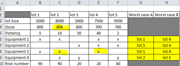
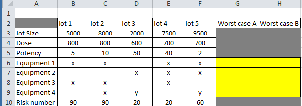
I have different lots made on different machines and the corresponding cells are marked x or y

In G6 I need to find out which lot has the largest risk number and smallest potency.
In H6 I need to find out which lot has the largest dose and smallest lot excluding the lot in G6.



For example in G6, lot 1 and lot 2 have highest risk number, then the second criterion should apply (smallest potency of lot 1 and lot 2). The output should be lot 1. Now in H6 formula should exclude lot 1 and look for other lots. So lot 4 and lot 5 have the highest dose and therefore the second criterion should apply (smallest lot size). The output should be lot 4.

I appreciate your help
P.S. I would have uploaded an Excel file but there is no option to upload a file.

 

[Special-K99]

You cant attach files on this forum. There are tools on this forum for adding small spreadsheet images

https://www.mrexcel.com/forum/about-board/508133-attachments.html

Or upload the file to an online storage site and post a link to it, though some people may not download the file for fear of viruses.

 

[Special-K99]

What happens if there's a tie in the final result, ie more than one lot has the same largest risk and smallest potency?
Could there be a tie or is this not possible?
Same goes for the value in H6.

in G6
=INDEX(B2:F2,1,MATCH(MIN(IF(B10:F10=MAX(B10:F10),B5:F5))
Array formula, use Ctrl-Shift-Enter

Second part is more tircky.

 

[Marcelo Branco]

Welcome to Mr Excel forum

Question:
Why the result in H6 should be lot 4?
Excluding the result in G6 (lot 1), lot 2 is the one with the largest Dose (800).
Could you clarify?

M.

 

[wideboydixon]

You'll need to check if this logic is valid but here's what I came up with. I hope you have MINIFS and MAXIFS ... !

Book1
	A	B	C	D	E	F	G	H
2		lot 1	lot 2	lot 3	lot 4	lot 5	Worst case A	Worst case B
3	lot Size	5000	8000	2000	7500	9500
4	Dose	800	800	600	700	700
5	Potency	5	10	50	40	2
6	Equipment 1	x	x		x	x	lot 1	lot 2
7	Equipment 2			x	x	x	lot 5	lot 4
8	Equipment 3	x	x		x		lot 1	lot 2
9	Equipment 4		x	y		y	lot 2	lot 5
10	Risk number	90	90	20	20	60
Sheet1

Cell Formulas
Range	Formula
G6	{=INDEX($B$2:$F$2,MIN(IF($B$5:$F$5=MINIFS($B$5:$F$5,$B6:$F6,"<>",$B$10:$F$10,MAXIFS($B$10:$F$10,$B6:$F6,"<>")),COLUMN($B6:$F6)-COLUMN($B6)+1)))}
H6	{=INDEX($B$2:$F$2,MIN(IF($B$3:$F$3=MINIFS($B$3:$F$3,$B6:$F6,"<>",$B$2:$F$2,"<>"&$G6,$B$4:$F$4,MAXIFS($B$4:$F$4,$B6:$F6,"<>",$B$2:$F$2,"<>"&$G6)),COLUMN($B6:$F6)-COLUMN($B6)+1)))}
Press CTRL+SHIFT+ENTER to enter array formulas.

WBD

 

[wideboydixon]

What happens if there's a tie in the final result, ie more than one lot has the same largest risk and smallest potency?
Could there be a tie or is this not possible?
Same goes for the value in H6.

in G6
=INDEX(B2:F2,1,MATCH(MIN(IF(B10:F10=MAX(B10:F10),B5:F5))
Array formula, use Ctrl-Shift-Enter

Second part is more tircky.

I think the "x" and "y" are significant. For example, lot 1 is not made on Equipment 1 and 4.

WBD

 

[Marcelo Branco]

If you do want to exclude all the lots with same risk than the risk of G6 (results in column G) maybe...

	A​	B​	C​	D​	E​	F​	G​	H​
1​
2​		lot 1​	lot 2​	lot 3​	lot 4​	lot 5​	Worst case A​	Worst case A​
3​	lot size​	5000​	8000​	2000​	7500​	9500​
4​	Dose​	800​	800​	600​	700​	700​
5​	Potency​	5​	10​	50​	40​	2​
6​	Equipment 1​	x​	x​		x​	x​	lot 1​	lot 4​
7​	Equipment 2​			x​	x​	x​	lot 5​	lot 4​
8​	Equipment 3​	x​	x​		x​		lot 1​	lot 4​
9​	Equipment 4​		x​	y​		y​	lot 2​	lot 5​
10​	Risk Number​	90​	90​	20​	20​	60​

Array formula in G6 copied down
=INDEX(B$2:F$2,MATCH(MAX(IF(B6:F6<>"",B$10:F$10-B$5:F$5/1000)),IF(B6:F6<>"",B$10:F$10-B$5:F$5/1000),0))
Ctrl+Shift+Enter

Array formula in H6 copied down
=INDEX(B$2:F$2,MATCH(MAX(IF(B6:F6<>"",IF(B$10:F$10<>INDEX(B$10:F$10,MATCH(G6,B$2:F$2,0)),B$4:F$4-B$3:F$3/(10^6)))),IF(B6:F6<>"",IF(B$10:F$10<>INDEX(B$10:F$10,MATCH(G6,B$2:F$2,0)),B$4:F$4-B$3:F$3/(10^6))),0))
Ctrl+Shift+Enter

Hope this helps

M.

 

[Med4040]

Welcome to Mr Excel forum

Question:
Why the result in H6 should be lot 4?
Excluding the result in G6 (lot 1), lot 2 is the one with the largest Dose (800).
Could you clarify?

M.

Thanks Marcelo,

So since the output in G6 is lot 1 (max risk number and lowest potency), lot 1 should be excluded in G6. Then, the remaining lots are lot 2, lot 3, lot 4 and lot 5. The lots with largest dose are lot 4 and lot5 but lot 4 has a smaller lot and therefore, the output should be lot 4.

 

[Marcelo Branco]

Thanks Marcelo,

So since the output in G6 is lot 1 (max risk number and lowest potency), lot 1 should be excluded in G6. Then, the remaining lots are lot 2, lot 3, lot 4 and lot 5. The lots with largest dose are lot 4 and lot5 but lot 4 has a smaller lot and therefore, the output should be lot 4.

Still not clear, at least for me.
Lot 2 has a dose of 800 that is larger than the doses of lots 4 and 5 (700).

M.

 

[Med4040]

If you do want to exclude all the lots with same risk than the risk of G6 (results in column G) maybe...

	A​	B​	C​	D​	E​	F​	G​	H​
1​
2​		lot 1​	lot 2​	lot 3​	lot 4​	lot 5​	Worst case A​	Worst case A​
3​	lot size​	5000​	8000​	2000​	7500​	9500​
4​	Dose​	800​	800​	600​	700​	700​
5​	Potency​	5​	10​	50​	40​	2​
6​	Equipment 1​	x​	x​		x​	x​	lot 1​	lot 4​
7​	Equipment 2​			x​	x​	x​	lot 5​	lot 4​
8​	Equipment 3​	x​	x​		x​		lot 1​	lot 4​
9​	Equipment 4​		x​	y​		y​	lot 2​	lot 5​
10​	Risk Number​	90​	90​	20​	20​	60​

<tbody>
</tbody>

Array formula in G6 copied down
=INDEX(B$2:F$2,MATCH(MAX(IF(B6:F6<>"",B$10:F$10-B$5:F$5/1000)),IF(B6:F6<>"",B$10:F$10-B$5:F$5/1000),0))
Ctrl+Shift+Enter

Array formula in H6 copied down
=INDEX(B$2:F$2,MATCH(MAX(IF(B6:F6<>"",IF(B$10:F$10<>INDEX(B$10:F$10,MATCH(G6,B$2:F$2,0)),B$4:F$4-B$3:F$3/(10^6)))),IF(B6:F6<>"",IF(B$10:F$10<>INDEX(B$10:F$10,MATCH(G6,B$2:F$2,0)),B$4:F$4-B$3:F$3/(10^6))),0))
Ctrl+Shift+Enter

Hope this helps

M.

Thanks so much Marcelo. You got the criteria exactly right. It is almost perfect but in H8, the output should be lot 2 because it has a larger dose (800) as compared to lot 4 (700)