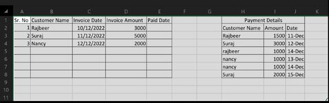
Automatically allocate the final paid date for the partially paid invoices

arrud14

New Member
Joined
Dec 17, 2022
Messages
14
Office Version
  1. 2021
  2. 2019
Platform
  1. Windows
Hii
I have a data set containing the invoice details and the details of recurring payment received from the customer and i want to allocate the final paid date for the every particular invoice calculating the sum of amount automatically
 

Attachments

  • IMG_20221217_234519.jpg
    IMG_20221217_234519.jpg
    229.7 KB · Views: 10
It is not clear to me. Your dates in column F all appear to be dates in 2023. Your dates in column K all appear to be dates in 2022.
For example, cell F3 shows this
1673489170910.png

45266 is the value for the date 6 December 2023.

So how did you get that clearance date for that cell?
 
Upvote 0

Excel Facts

Convert text numbers to real numbers
Select a column containing text numbers. Press Alt+D E F to quickly convert text to numbers. Faster than "Convert to Number"
It is not clear to me. Your dates in column F all appear to be dates in 2023. Your dates in column K all appear to be dates in 2022.
For example, cell F3 shows this
View attachment 82591
45266 is the value for the date 6 December 2023.

So how did you get that clearance date for that cell?
That was an mistake as i have manually put the dates in the column F but i want to allocate the payments dates in the COULMN F calculating the sum of invoices and payments
As shown in the table from 5th Dec 2022 to 6th Dec 2022 there are three invoices for rajan pal (2591,5432,4806) the total of which is 12829 and then on 6th Dec 2022 Rajan Pal Paid 12100 so the amount of rs 729 was outstanding from the invoice no. 3rd ( 4806 ) which gets cleared on next payment which is 10th Dec
 
Upvote 0
That was an mistake
OK, I assume all those column F dates were meant to be 2022.

See if this works for you.

arrud14.xlsm
BCDEFHIJKL
2Invoice DateInvoice AmountInvoice No.NamesClearence dateFosBankingDateBank
305.12.2022259139453074RAJAN PAL06-Dec-22CHANDAN330008-Dec-22PUNB
406.12.2022543239468693RAJAN PAL06-Dec-22CHANDAN595011-Dec-22PUNB
506.12.2022480639460801RAJAN PAL10-Dec-22CHANDAN600012-Dec-22PUNB
607.12.2022255039503179RAJAN PAL10-Dec-22CHANDAN390013-Dec-22PUNB
708.12.2022330039542391CHANDAN08-Dec-22CHANDAN800014-Dec-22PUNB
809.12.2022344439566311CHANDAN11-Dec-22RAJAN PAL1210006-Dec-22PUNB
909.12.2022250539566584CHANDAN11-Dec-22RAJAN PAL608210-Dec-22PUNB
1009.12.2022275139574859RAJAN PAL10-Dec-22RAJAN PAL1142112-Dec-22PUNB
1112.12.2022341139608264CHANDAN12-Dec-22RAJAN PAL371113-Dec-22PUNB
1212.12.2022480539608111CHANDAN13-Dec-22
1312.12.2022270039625463CHANDAN14-Dec-22
1412.12.2022360039611283CHANDAN14-Dec-22
1512.12.2022422539603022RAJAN PAL12-Dec-22
1612.12.2022290239603295RAJAN PAL12-Dec-22
1712.12.2022429439603153RAJAN PAL12-Dec-22
1813.12.2022390039685842CHANDANnot paid
1913.12.2022371139671011RAJAN PAL13-Dec-22
Sheet1
Cell Formulas
RangeFormula
F3:F19F3=LET(n,FILTER(J$3:K$11,I$3:I$11=E3,""),XLOOKUP(SUMIF(E$3:E3,E3,C$3:C3),INDEX(SCAN(0,INDEX(n,0,1),LAMBDA(t,s,t+s)),0,1),INDEX(n,0,2),"not paid",1))
 
Upvote 0
I am using excel 2019 and it doesnt accepting/ supporting FILTER formula
 
Upvote 0
OK, I assume all those column F dates were meant to be 2022.

See if this works for you.

arrud14.xlsm
BCDEFHIJKL
2Invoice DateInvoice AmountInvoice No.NamesClearence dateFosBankingDateBank
305.12.2022259139453074RAJAN PAL06-Dec-22CHANDAN330008-Dec-22PUNB
406.12.2022543239468693RAJAN PAL06-Dec-22CHANDAN595011-Dec-22PUNB
506.12.2022480639460801RAJAN PAL10-Dec-22CHANDAN600012-Dec-22PUNB
607.12.2022255039503179RAJAN PAL10-Dec-22CHANDAN390013-Dec-22PUNB
708.12.2022330039542391CHANDAN08-Dec-22CHANDAN800014-Dec-22PUNB
809.12.2022344439566311CHANDAN11-Dec-22RAJAN PAL1210006-Dec-22PUNB
909.12.2022250539566584CHANDAN11-Dec-22RAJAN PAL608210-Dec-22PUNB
1009.12.2022275139574859RAJAN PAL10-Dec-22RAJAN PAL1142112-Dec-22PUNB
1112.12.2022341139608264CHANDAN12-Dec-22RAJAN PAL371113-Dec-22PUNB
1212.12.2022480539608111CHANDAN13-Dec-22
1312.12.2022270039625463CHANDAN14-Dec-22
1412.12.2022360039611283CHANDAN14-Dec-22
1512.12.2022422539603022RAJAN PAL12-Dec-22
1612.12.2022290239603295RAJAN PAL12-Dec-22
1712.12.2022429439603153RAJAN PAL12-Dec-22
1813.12.2022390039685842CHANDANnot paid
1913.12.2022371139671011RAJAN PAL13-Dec-22
Sheet1
Cell Formulas
RangeFormula
F3:F19F3=LET(n,FILTER(J$3:K$11,I$3:I$11=E3,""),XLOOKUP(SUMIF(E$3:E3,E3,C$3:C3),INDEX(SCAN(0,INDEX(n,0,1),LAMBDA(t,s,t+s)),0,1),INDEX(n,0,2),"not paid",1))
I am using excel 2019 and it doesnt accepting/ supporting FILTER formula
 
Upvote 0
Could you pls let me know how can i do rhe same with excel 2019
While I am thinking about that, could you please fix your profile details? (so future helpers do not waste their times developing a solution that does not work for you)
 
Upvote 0
While I am thinking about that, could you please fix your profile details? (so future helpers do not waste their times developing a solution that does not work for you)
Sir i really apologize for your inconvenience but i use both versions of excel 2019 in my official laptop and excel 2021 in my personal laptop that why i just want you to let me know how i can do the same with excel 2019 if possible
 
Upvote 0
i use both versions of excel 2019 in my official laptop and excel 2021 in my personal laptop
In that case mark them both in your account details now ..
1673652123939.png


.. and in future when you ask a question if it needs to work in the older version, say so in the first post of the thread.
 
Upvote 0

Forum statistics

Threads
1,215,135
Messages
6,123,239
Members
449,093
Latest member
Vincent Khandagale

We've detected that you are using an adblocker.

We have a great community of people providing Excel help here, but the hosting costs are enormous. You can help keep this site running by allowing ads on MrExcel.com.
Allow Ads at MrExcel

Which adblocker are you using?

Disable AdBlock

Follow these easy steps to disable AdBlock

1)Click on the icon in the browser’s toolbar.
2)Click on the icon in the browser’s toolbar.
2)Click on the "Pause on this site" option.
Go back

Disable AdBlock Plus

Follow these easy steps to disable AdBlock Plus

1)Click on the icon in the browser’s toolbar.
2)Click on the toggle to disable it for "mrexcel.com".
Go back

Disable uBlock Origin

Follow these easy steps to disable uBlock Origin

1)Click on the icon in the browser’s toolbar.
2)Click on the "Power" button.
3)Click on the "Refresh" button.
Go back

Disable uBlock

Follow these easy steps to disable uBlock

1)Click on the icon in the browser’s toolbar.
2)Click on the "Power" button.
3)Click on the "Refresh" button.
Go back
Back
Top