Calculate total hours for week based on total time of each day

GodzFire

New Member
Joined
Apr 30, 2018
Messages
20
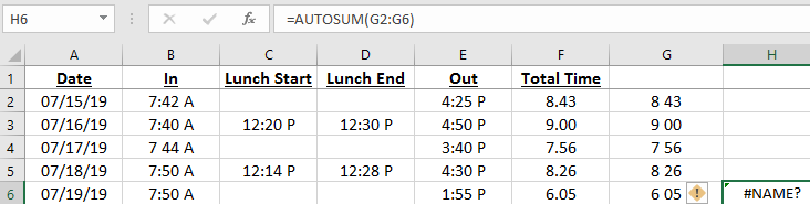
I have the following table I use to keep track of my work hours:
tcyEOg4.png


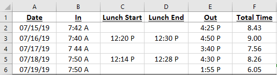
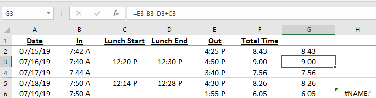
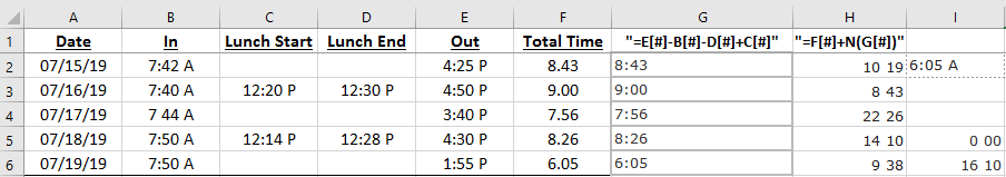
I calculated the Total Time column with the following formula (example row 3) which takes the lunch time (D3-C3) and subtracts it from the total In-Out time (E3-B3): =TEXT((E3-B3)-(D3-C3), "h.mm")

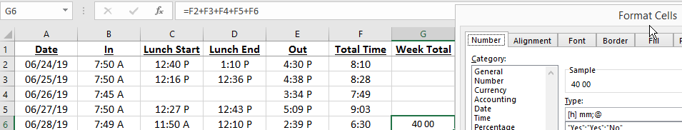
This works fine, but I also have to make sure I am under 40 hours per week, so I want to automatically total up the hours as well and have it output in a cell in Column G. I tried using an Autosum, =AUTOSUM(F2:F6), but it comes back with a #NAME ? error.

I'm not sure what I'm doing wrong and feel pretty dumb I can't figure this out. Can anyone assist? Feel free to re-do my formulas or do something different if it's easier/simpler. Thank you very much.
 

Excel Facts

What do {} around a formula in the formula bar mean?
{Formula} means the formula was entered using Ctrl+Shift+Enter signifying an old-style array formula.
Hi,

Instead of text just use =E3-B3-D3+C3 and change the number format for column G to h:mm then your sum will work.
 
Last edited:
Upvote 0
Hmmm, why I can't edit my own post?


Hi,

Instead of text just use =E3-B3-D3+C3 and change the number format for column G to h:mm then your sum will work.

Anyway, I did try what you mentioned in a new column G and then the total in H, but I get the same #NAME issue:
U7ev3PG.png

ym0ROuZ.png
 
Upvote 0
I tried but - see if this works.


Excel 2013/2016
ABCDEFG
1DateInLunch StartLunch EndOutTotal TimeTotal Time(Hrs)
215-07-197:42 AM4:25 PM8:43 AM17:12
316-07-197:40 AM12:20 PM12:30 PM4:50 PM9:00 AM0:00
417-07-197:44 AM3:40 PM7:56 AM22:24
518-07-197:50 AM12:14 PM12:28 PM4:30 PM8:26 AM10:24
619-07-197:50 AM1:55 PM6:05 AM2:00
Sheet2
Cell Formulas
RangeFormula
F2=TEXT(E2-B2,"H:M")-TEXT(D2-C2,"H:M")*24
F3=TEXT(E3-B3,"H:M")-TEXT(D3-C3,"H:M")
F4=TEXT(E4-B4,"H:M")-TEXT(D4-C4,"H:M")
F5=TEXT(E5-B5,"H:M")-TEXT(D5-C5,"H:M")
F6=TEXT(E6-B6,"H:M")-TEXT(D6-C6,"H:M")
G2=F2*24
G3=F3*24
G4=F4*24
G5=F5*24
G6=F6*24
G8=SUM(G2:G7)


Thanks Muz
 
Upvote 0
2 alternatives that you can try


Excel 2010
ABCDEFG
1DateInLunch StartLunch EndOutTotal TimeTotal Time(Hrs)
215-Jul-197:42 AM4:25 PM08:438:43
316-Jul-197:40 AM12:20 PM12:30 PM4:50 PM09:0017:43
417-Jul-197:44 AM3:40 PM07:5625:39
518-Jul-197:50 AM12:14 PM12:28 PM4:30 PM08:2634:05
619-Jul-197:50 AM1:55 PM06:0540:10
7
8Column G custom number format "[h]:mm"40:00Regular40:00
9Overtime0:10
10Total$22.00$885.50
11
12DateInLunch StartLunch EndOutTotal TimeTotal Time(Hrs)
1315-Jul-197:42 AM4:25 PM8.728.72
1416-Jul-197:40 AM12:20 PM12:30 PM4:50 PM9.0017.72
1517-Jul-197:44 AM3:40 PM7.9325.65
1618-Jul-197:50 AM12:14 PM12:28 PM4:30 PM8.4334.08
1719-Jul-197:50 AM1:55 PM6.0840.17
18Regular40.00
19Overtime0.17
20$885.50
21
4b
Cell Formulas
RangeFormula
F2=(C2-B2+E2-D2)
F13=(C13-B13+E13-D13)*24
G2=F2+N(G1)
G8=MIN(E8,G6)
G9=G6-G8
G10=G8*24*D10+G9*24*D10*1.5
G13=F13+N(G12)
G18=MIN(40,G17)
G19=G17-G18
G20=G18*D10+G19*1.5*D10
 
Upvote 0
Yey Dave awesome,

“Mine is silly”.

I was wondering when I manually add his total hours, =8.43+9.00+7.56+8.26+6.05 gives 39.30 hrs. But when I select (F2:F6) excel says its 40.10 hrs. How is it possible?
 
Last edited:
Upvote 0
2 alternatives that you can try

Excel 2010
ABCDEFG
1DateInLunch StartLunch EndOutTotal TimeTotal Time(Hrs)
215-Jul-197:42 AM4:25 PM08:438:43
316-Jul-197:40 AM12:20 PM12:30 PM4:50 PM09:0017:43
417-Jul-197:44 AM3:40 PM07:5625:39
518-Jul-197:50 AM12:14 PM12:28 PM4:30 PM08:2634:05
619-Jul-197:50 AM1:55 PM06:0540:10
7
8Column G custom number format "[h]:mm"40:00Regular40:00
9Overtime0:10
10Total$22.00$885.50
11
12DateInLunch StartLunch EndOutTotal TimeTotal Time(Hrs)
1315-Jul-197:42 AM4:25 PM8.728.72
1416-Jul-197:40 AM12:20 PM12:30 PM4:50 PM9.0017.72
1517-Jul-197:44 AM3:40 PM7.9325.65
1618-Jul-197:50 AM12:14 PM12:28 PM4:30 PM8.4334.08
1719-Jul-197:50 AM1:55 PM6.0840.17
18Regular40.00
19Overtime0.17
20$885.50
21

<tbody>
</tbody>
4b

Worksheet Formulas
CellFormula
F2=(C2-B2+E2-D2)
G2=F2+N(G1)
G8=MIN(E8,G6)
G9=G6-G8
G10=G8*24*D10+G9*24*D10*1.5
F13=(C13-B13+E13-D13)*24
G13=F13+N(G12)
G18=MIN(40,G17)
G19=G17-G18
G20=G18*D10+G19*1.5*D10

<tbody>
</tbody>

<tbody>
</tbody>

Dave would you be able to upload a copy of the excel sheet you got it to work under? I'm still having issues where it's not doing what you are showing for some reason. For example here's some attempts at doing it on mine:
dM5WGVX.png
 
Upvote 0
F2:F6 are hours and minutes; f2:F6 yields 40 hours and 10 minutes. Your formula is using decimals 8.43 is not 8 hours and 43 minutes.

Copy the example as posted and entry the formulas. Copy the formulas down as required.
 
Upvote 0
I somehow stumbled onto the formula "=F2+F3+F4+F5+F6" that when put in G6 and formatted with "[h] mm;@", gets exactly what I need!
H68gBYj.png
 
Upvote 0

Forum statistics

Threads
1,215,669
Messages
6,126,120
Members
449,293
Latest member
yallaire64

We've detected that you are using an adblocker.

We have a great community of people providing Excel help here, but the hosting costs are enormous. You can help keep this site running by allowing ads on MrExcel.com.
Allow Ads at MrExcel

Which adblocker are you using?

Disable AdBlock

Follow these easy steps to disable AdBlock

1)Click on the icon in the browser’s toolbar.
2)Click on the icon in the browser’s toolbar.
2)Click on the "Pause on this site" option.
Go back

Disable AdBlock Plus

Follow these easy steps to disable AdBlock Plus

1)Click on the icon in the browser’s toolbar.
2)Click on the toggle to disable it for "mrexcel.com".
Go back

Disable uBlock Origin

Follow these easy steps to disable uBlock Origin

1)Click on the icon in the browser’s toolbar.
2)Click on the "Power" button.
3)Click on the "Refresh" button.
Go back

Disable uBlock

Follow these easy steps to disable uBlock

1)Click on the icon in the browser’s toolbar.
2)Click on the "Power" button.
3)Click on the "Refresh" button.
Go back
Back
Top