Calculating a percentage in a pivot table

[nielf]

I'm trying figure out how to create a calculated field which will return the hit rate based on awarded/lost opportunities.

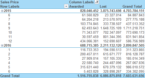
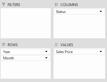
I have created a pivot table with some dummy data looking like this:

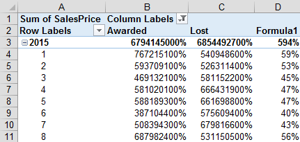
I'm trying to to create field that will return the hit rate (Awarded / Awarded + Lost) for each month. I must admit I'm lost here. Do I need to add any dummy columns to my source data to be able to do this? I've tried working with the SUMIF function without any luck.

I hope you can point me in the right direction.

 

[BGY23]

Hi Its realtively straight forward.

Click in your pivit table, Go to the analze tab and click Field, Item sets,
From the drop down list select calculated fields
In the pop up

Name Give the field a name i.e % awarded.
Formula =Awarded /(Awarded +Lost )

Click ok and format the column to show percentage

 

[nielf]

To do that I have to create the Awarded and Lost columns as 'dummy columns' in my source data as they are not actual columns (I cannot select them from the field list in the 'insert calculated field' dialog box'.

However, that might be easier to work with than ending up with a long formula.

Thanks.

 

[RoryA]

Sounds like you want a calculated item then, not a calculated field. From a performance point of view, you may find that the additional columns in the source data are preferable.

 

[BGY23]

You use the awarded and Lost fields already in your pivot table in the diagram above.

 

[nielf]

Thanks for the input. I will try to mess around with the calculated item/field options and see if I can figure out what is the best solution.

What I'm trying to achieve is a pivot chart looking like the one below. However, I think it might be a problem creating a stacked chart with a line chart as a pivot chart.

 

[RoryA]

You can do that with a pivot chart - it's an allowed combination.

 

[nielf]

BGY23,

I have uploaded an example workbok. Can you show me how you would create the calculated field/item from this dummy workbook?

https://www.dropbox.com/s/em426kfmyv1xjbr/DummyData.xlsx?dl=1

 

[BGY23]

Hi There, I have a solution. Its a bit tricky but it will work.

Set out your pivot table with the Status as a field item and the months as column headings.

Click in the pivot table Rows area (where the status is listed). Now click analyze on the ribbon and Field Items set and caculated item.
In the drop down box name the item % awarded. in the formula field pu this formula = (Awarded/(Awarded+Lost)) click ok

Now go back to your pivot table and move staus to the columns area and Months to the row area and you should see.

Rows = Year and Months

COls = Awarded, lost, % awarded. It will show a grand total for awarded and Lost too.

Goodn luck

 

[nielf]

Thanks for the reply, BGY23.

I have two issues:

1. When I try to change the number format for the calculated item to percentage the two other columns (awarded and lost) changes as well. Is there any way to avoid that?

I guess I could change the format for the entire column D but that's not a very flexible solution if I need to add more columns.

2. This solution works fine with my dummy data but when i try to replicate it in my actual working data I get the error below:

It's the same fields in my working data as in the dummy data. Could it be something in the source data that's causing this error?

If I can't get it working this way I guess I could create two helper columns in my source data and use them instead as a workaround.