Hello all MrExcel experts,
I try to fasten my vba code posted below, already use screenupdating false function, empty cache. Currently I need 3 steps to use LinEst function for an Arr:
Step1, write Arr to Range
Step2, get Range
Step3, use Range in LinEst
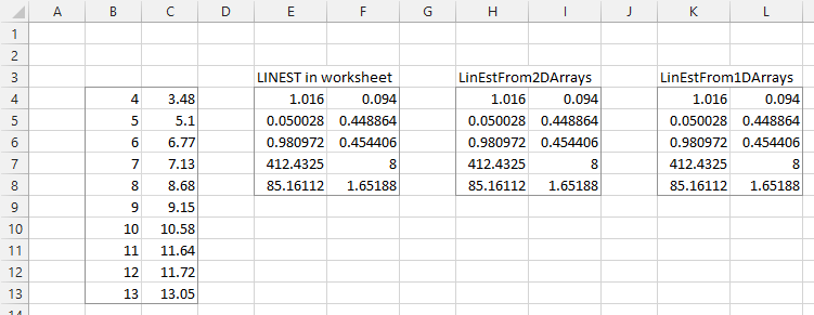
I want to know, can Excel VBA LinEst using dynamic Arr directly? Like "z1 = Application.WorksheetFunction.LinEst(Arr(z, 3), , False, True).
Other comments on optimizing speed also highly appreciated")
------------------------------------------------------
Option Base 1
Sub faster()
Application.ScreenUpdating = False
Dim x, y, z As Integer
Dim x1, x2, x3 As Double
For x = 1 To 100
Application.ScreenUpdating = True
End Sub
I try to fasten my vba code posted below, already use screenupdating false function, empty cache. Currently I need 3 steps to use LinEst function for an Arr:
Step1, write Arr to Range
Step2, get Range
Step3, use Range in LinEst
I want to know, can Excel VBA LinEst using dynamic Arr directly? Like "z1 = Application.WorksheetFunction.LinEst(Arr(z, 3), , False, True).
Other comments on optimizing speed also highly appreciated
------------------------------------------------------
Option Base 1
Sub faster()
Application.ScreenUpdating = False
Dim x, y, z As Integer
Dim x1, x2, x3 As Double
For x = 1 To 100
For y = 1 To 100
ReDim Arr(1 To Range("a" & x).End(xlDown).Row, 1 To 3)
For z = 1 To 100
If ... Then
x1 = ......
Else If ... Then
x1 = .......
Else
x1 = ......
End If
Arr(z, 1) = x1
If ... Then
x2 = ......
Else If ... Then
x2 = .......
Else
x2 = ......
End If
Arr(z, 2) = x2
If Arr(z, 1)...And Arr(z, 2)... Then
x3 = ......
Else If Arr(z, 1)...And Arr(z, 2)... Then
x3 = .......
Else
x3 = ......
End If
Arr(z, 3) = x3
Next z
Range("b1:b" & Range("a" & x).End(xlDown).Row) = Application.Index(Arr, , 3) 'Step1, write arr to range
Dim y1, z1 As Variant
y1 = Range("b1:b" & Range("a" & x).End(xlDown).Row).Value 'Step2, get range
z1 = Application.WorksheetFunction.LinEst(y1, , True, True) 'Step3, use range in LinEst
Cells(1, 3) = z1(3, 1)
Erase Arr
Erase Arr
Set z1 = Nothing
Next y
Next xApplication.ScreenUpdating = True
End Sub