Cohort Waterfall by account count

[robbied13]

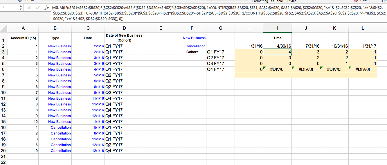
I am trying to build out a waterfall that will count how many customers we have based on what time they became a customer. The plan is to count the account IDs if they are new business and remove them if they have been cancelled. The issue is an account can have numerous opportunities marked as new business. As seen in the example of data provided on the left, account "1" has several new business opportunities but it should only be counted as 1 account. The table on the right is what I am trying to get to based on the data provided. Time is the x axis and the quarter the customer was new is the y axis. The values in the table are just hardcodes as I'm struggling with the equations. Any help would be much appreciated

---

Account ID (15)	Type	Date of New Business (Cohort)	Cancellation Date			Time
1	New Business	Q1 FY17				Q1 FY17	Q2 FY17	Q3 FY17	Q4 FY17
1	New Business	Q1 FY17		Cohort	Q1 FY17	4	3	2	1
2	New Business	Q1 FY17			Q2 FY17		2	2	1
3	New Business	Q1 FY17			Q3 FY17			1	1
4	New Business	Q1 FY17			Q4 FY17				3
5	New Business	Q2 FY17				4	5	5	6
5	New Business	Q2 FY17
6	New Business	Q2 FY17
7	New Business	Q3 FY17
8	New Business	Q4 FY17
8	New Business	Q4 FY17
8	New Business	Q4 FY17
9	New Business	Q4 FY17
10	New Business	Q4 FY17
1	Cancellation	Q1 FY17	Q2 FY17
2	Cancellation	Q1 FY17	Q3 FY17
3	Cancellation	Q1 FY17	Q4 FY17
6	Cancellation	Q2 FY17	Q4 FY17

<colgroup><col><col><col><col><col span="6"></colgroup><tbody>
</tbody>

<style><!--table {mso-displayed-decimal-separator:"\."; mso-displayed-thousand-separator:"\,";}@page {margin:.75in .7in .75in .7in; mso-header-margin:.3in; mso-footer-margin:.3in;}tr {mso-height-source:auto;}col {mso-width-source:auto;}br {mso-data-placement:same-cell;}td {padding-top:1px; padding-right:1px; padding-left:1px; mso-ignoreadding; color:windowtext; font-size:10.0pt; font-weight:400; font-style:normal; text-decoration:none; font-family:Arial; mso-generic-font-family:auto; mso-font-charset:0; mso-number-format:General; text-align:general; vertical-align:bottom; border:none; mso-background-source:auto; mso-pattern:auto; mso-protection:locked visible; white-space:nowrap; mso-rotate:0;}.xl65 {font-family:Arial, sans-serif; mso-font-charset:0;}.xl66 {font-size:8.0pt; font-weight:700; font-family:Arial, sans-serif; mso-font-charset:0; text-align:center; vertical-align:middle; mso-protection:unlocked visible;}.xl67 {background:#FFF2CC; mso-pattern:black none;}.xl68 {border-top:none; border-right:none; border-bottom:.5pt solid windowtext; border-left:none; background:#FFF2CC; mso-pattern:black none;}--></style>

 

[robbied13]

Where I'm at so far for the Q1 FY17...

First, I did the following formula to get unique ids for account numbers. It spit out 10, which is the total number of accounts in the sample
=SUMPRODUCT(1/COUNTIF(A2:A19,A2:A19))

Second, i just have a countifs formula to get the number of new business lines that were for Q1 FY17, This gives me 5.
=COUNTIFS(B2:B19,Sheet2!A1,C2:C19,F3)

What I'm trying to figure out is how to combine the formulas so that Q1 FY17 is 4.

 

[robbied13]

Combining Unique Values with multiple criteria array formula

I had posted elsewhere but heres a new thread just due to the amount of work I've put in.

I think I'm really close on this but could use some help. I'm trying to get a rolling count of all of our accounts. The table is what I'm trying to fill in and the detail is below. For some reason the array formula works in every cell except the Q4 FY17 row and I can't understand why. I've copied the formula in here. It basically say count all new business that came in within the fiscal quarter less any accounts that cancelled within the same quarter.

I posted the screen shot as well as the detail in text if either are helpful

{=SUM(IF(($F$1=$B$2:$B$20)*($C$2:$C$20<=I$2)*($D$2:$D$20>=$H$2)*($G3=$D$2:$D$20), 1/COUNTIFS($B$2:$B$20, $F$1, $A$2:$A$20, $A$2:$A$20, $C$2:$C$20, "<="&I$2, $C$2:$C$20, ">="&$H$2, $D$2:$D$20, $G3)), 0)-SUM(IF(($F$2=$B$2:$B$20)*($C$2:$C$20<=I$2)*($D$2:$D$20>=$H$2)*($G3=$D$2:$D$20), 1/COUNTIFS($B$2:$B$20, $F$2, $A$2:$A$20, $A$2:$A$20, $C$2:$C$20, "<="&I$2, $C$2:$C$20, ">="&$H$2, $D$2:$D$20, $G3)), 0)}

<style><!--table {mso-displayed-decimal-separator:"\."; mso-displayed-thousand-separator:"\,";}@page {margin:.75in .7in .75in .7in; mso-header-margin:.3in; mso-footer-margin:.3in;}tr {mso-height-source:auto;}col {mso-width-source:auto;}br {mso-data-placement:same-cell;}td {padding-top:1px; padding-right:1px; padding-left:1px; mso-ignoreadding; color:windowtext; font-size:10.0pt; font-weight:400; font-style:normal; text-decoration:none; font-family:Arial; mso-generic-font-family:auto; mso-font-charset:0; mso-number-format:General; text-align:general; vertical-align:bottom; border:none; mso-background-source:auto; mso-pattern:auto; mso-protection:locked visible; white-space:nowrap; mso-rotate:0;}.xl65 {color:blue; font-size:8.0pt; font-family:Arial, sans-serif; mso-font-charset:0; text-align:right; vertical-align:middle; mso-protection:unlocked visible;}.xl66 {font-family:Arial, sans-serif; mso-font-charset:0;}.xl67 {font-size:8.0pt; font-weight:700; font-family:Arial, sans-serif; mso-font-charset:0; text-align:center; vertical-align:middle; mso-protection:unlocked visible;}.xl68 {background:#FFF2CC; mso-pattern:black none;}.xl69 {border-top:none; border-right:none; border-bottom:.5pt solid windowtext; border-left:none; background:#FFF2CC; mso-pattern:black none;}.xl70 {mso-number-format:"Short Date";}.xl71 {font-family:Arial, sans-serif; mso-font-charset:0; mso-number-format:"Short Date";}.xl72 {color:blue; font-size:8.0pt; font-family:Arial, sans-serif; mso-font-charset:0; text-align:right; vertical-align:middle; mso-protection:unlocked visible;}--></style>

New Business			Time
Cancellation		1/31/16	4/30/16	7/31/16	10/31/16	1/31/17
Cohort	Q1 FY17	0	4	3	2	1
	Q2 FY17	0	0	2	2	1
	Q3 FY17	0	0	0	1	1
	Q4 FY17	0	#DIV/0!	#DIV/0!	#DIV/0!	#DIV/0!

<!--StartFragment--> <colgroup><col width="87" span="7" style="width:65pt"> </colgroup><tbody>
<!--EndFragment--></tbody>

Account ID (15)	Type	Date	Date of New Business (Cohort)
1	New Business	2/1/16	Q1 FY17
1	New Business	2/1/16	Q1 FY17
2	New Business	3/1/16	Q1 FY17
3	New Business	3/1/16	Q1 FY17
4	New Business	4/1/16	Q1 FY17
5	New Business	5/1/16	Q2 FY17
5	New Business	5/1/16	Q2 FY17
6	New Business	6/1/16	Q2 FY17
7	New Business	8/1/16	Q3 FY17
8	New Business	11/1/16	Q4 FY17
8	New Business	11/1/16	Q4 FY17
8	New Business	11/1/16	Q4 FY17
9	New Business	12/1/16	Q4 FY17
10	New Business	1/1/16	Q4 FY17
1	Cancellation	5/1/16	Q1 FY17
2	Cancellation	8/1/16	Q1 FY17
3	Cancellation	11/1/16	Q1 FY17
6	Cancellation	12/1/16	Q2 FY17
9	Cancellation	12/1/16	Q4 FY17

<colgroup><col><col span="2"><col></colgroup><tbody>
</tbody>

 

[Macropod]

Re: Combining Unique Values with multiple criteria array formula

Kindly don't start multiple threads on the same topic. Threads merged.