Combination Filtering

[HarperMA]

I have 2 sheets Form_ERR and DataBase_ERR.

Form_ERR has: -
Cell L11 - where a number can be entered
Cell L14 - dropdown selection containing Names
Cell L16 - dropdown selection containing Categories
Cell L18 - dropdown selection contain Departments
Cell L20 - dropdown selection containing Status

DataBase_ERR has: -
Table - DataBase_ERR (range C24:N1000)
Header C - [Status]
Header D - [ERR]
Header E - [Description]
Header F - [Date In]
Header G - [Target]
Header H - [Dept]
Header I - [Requester]
Header J - [Market]
Header K - [Classification]
Header L - [Priority]
Header M - [Engineer]
Header N - [Completion Date]

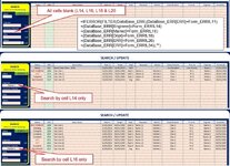
I have a formula (below) that filters the table (DataBase_ERR) if one of the cells above contains a value (only one cell contains a value at any one time).
=FILTER(DataBase_ERR,(DataBase_ERR[ERR]=Form_ERR!L11)+(DataBase_ERR[Engineer]=Form_ERR!L14)+(DataBase_ERR[Market]=Form_ERR!L16)+(DataBase_ERR[Dept]=Form_ERR!L18)+(DataBase_ERR[ERR]=Form_ERR!L26)+(DataBase_ERR[ERR]=Form_ERR!L34))

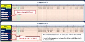
This above formula works fine, but I now need to combine an additional filter that will do the same as above but also Filter if Cell L14 and Cell L20 have values. The formula I have for this is: -
=IFERROR(FILTER(DataBase_ERR,((DataBase_ERR[Engineer]=L14)+(DataBase_ERR[Market]=L16)+(DataBase_ERR[Dept]=L18))*(DataBase_ERR[Engineer]=L14)*(DataBase_ERR[Status]=L20)),"")

This formula will give me the filter results I want but if I leave Cell L20 blank then I get no results at all.

I'm a keen learner but very much a noob, so any help would be gratefully received.
Mark.

 

[StephenCrump]

Welcome to the Forum!

This formula will give me the filter results I want but if I leave Cell L20 blank then I get no results at all.

I'm not completely clear on the one cell / two cells containing values.

But in general terms, if you want to filter only when a non-blank filter value is specified, you can change a term like this:

(DataBase_ERR[Status]=L20) 

to 

IF(L20="",1,DataBase_ERR[Status]=L20)

 

[HarperMA]

Hi Stephen,

 

[HarperMA]

Hi Stephen,

I couldn't get you IF(L20= etc to work so I have uploaded a couple of screen grabs that hopefully may help explain in more detail.
In the yellow search box there are 3 options for me to search by (using dropdown menus).
* Engineer
* Market
* Dept
* Status

I can select an option from the dropdown menu (eg. Engineer - would give me Name 1)
My filter formula will then summaries all jobs by this name.

Again I can summaries the list if I use either of the other dropdown menus * Market, * Dept * Status.
What I need to do is also summaries if I have * Engineer and * Status selected at the same time.

As you can see from the second image my current formula does not do this.

Hope the above helps.

Many thyanks
Mark.

 

[StephenCrump]

... so I have uploaded a couple of screen grabs that hopefully may help explain in more detail.

Unfortunately screenshots aren't much help. The best way to post an example is to use the XL2BB add-in, as I have done below. That way we can copy/paste direct into a workbook.

Here's what I had in mind:

	A	B	C	D	E
1
2		Name	Status	Class	Code
3		A	Yes	1	101
4		A	Yes	2	102
5		B	Yes	3	103
6		C	No	3	104
7		B	No	2	105
8		D	Yes	1	106
9		C	No	1	107
10		A	Yes	2	108
11
12		Filter
13		A		2
14
15		Results
16		A	Yes	2	102
17		A	Yes	2	108
Sheet1

Cell Formulas
Range	Formula
B16:E17	B16	=FILTER(MyTable,IF(B13="",1,MyTable[Name]=B13)*IF(C13="",1,MyTable[Status]=C13)*IF(D13="",1,MyTable[Class]=D13))
Dynamic array formulas.

I'm not clear why you're adding your filters?

Multiplying is for AND. Adding is for OR. For example, to filter by Name="A" OR Class=2:

	A	B	C	D	E
1
2		Name	Status	Class	Code
3		A	Yes	1	101
4		A	Yes	2	102
5		B	Yes	3	103
6		C	No	3	104
7		B	No	2	105
8		D	Yes	1	106
9		C	No	1	107
10		A	Yes	2	108
11
12		Results
13		A	Yes	1	101
14		A	Yes	2	102
15		B	No	2	105
16		A	Yes	2	108
Sheet1

Cell Formulas
Range	Formula
B13:E16	B13	=FILTER(MyTable,(MyTable[Name]="A")+(MyTable[Class]=2))
Dynamic array formulas.

 

[HarperMA]

Hi Stephen,
Again, thanks very much for your update.
Unfortunately, I don't have the access rights to install add-ons.

However, after some tinkering with your formula's above I now have the formula that works for me (see below).

=IFERROR(FILTER(DataBase_ERR,IF(L14="",1,DataBase_ERR[Engineer]=L14)*IF(L16="",1,DataBase_ERR[Market]=L16)*IF(L18="",1,DataBase_ERR[Dept]=L18)*IF(L14="",1,Database_ERR[Engineer]=L14)*IF(L20="",1,DataBase_ERR[Status]=L20)),"")

I will try to upload an example workbook, in case it proves helpful to anyone else.

In the mean time, if the above formula is of use for anyone else please see below.

Workbook
* Sheet 1
* Sheet 2

 

[HarperMA]

Hi Stephen,
Again, thanks very much for your update.
Unfortunately, I don't have the access rights to install add-ons.

However, after some tinkering with your formula's above I now have the formula that works for me (see below).

=IFERROR(FILTER(DataBase_ERR,IF(L14="",1,DataBase_ERR[Engineer]=L14)*IF(L16="",1,DataBase_ERR[Market]=L16)*IF(L18="",1,DataBase_ERR[Dept]=L18)*IF(L14="",1,Database_ERR[Engineer]=L14)*IF(L20="",1,DataBase_ERR[Status]=L20)),"")

I will try to upload an example workbook, in case it proves helpful to anyone else.

In the mean time, if the above formula is of use for anyone else please see below.

Workbook
* Sheet 1
* Sheet 2

Sheet 1 is where the search cells A1, A2, A3 & A4 are located.
Sheet 2 is where the TABLE is located.
The TABLE contains 4 columns [ENGINEER], [MARKET], [DEPT] & [STATUS]

So,

=IFERROR(FILTER(TABLE,IF(A1="",1,TABLE[Engineer]=A1)*IF(A2="",1,TABLE[Market]=A2)*IF(A3="",1,TABLE[Dept]=A3)*IF(A4="",1,TABLE[Engineer]=A4)*IF(A5="",1,TABLE[Status]=A4)),"")


as a bonus, I've also added a Choosecols to filter just [ENGINEER] & [STATUS]

=IFERROR(CHOOSECOLS(FILTER(TABLE,IF(A1="",1,TABLE[Engineer]=A1)*IF(A2="",1,TABLE[Market]=A2)*IF(A3="",1,TABLE[Dept]=A3)*IF(A4="",1,TABLE[Engineer]=A4)*IF(A5="",1,TABLE[Status]=A4)),""),1,4)


Many, Many thanks for you help.
Mark.

 

[StephenCrump]

Excellent, I'm glad you got it working.

If you do want to post a workbook (making sure it doesn't contain confidential or sensitive information, of course), you'll need to upload to a drop box site, and include the link in your post to this forum.