Combine Calculate in a cells with several calculate in that cell and after that another calculate based on that cell

[Unexpc]

Hi guys
i have main problem and if you solve this, solve my main problem and helped me to calculate any of numbers that i do this in many hours
this is my problem
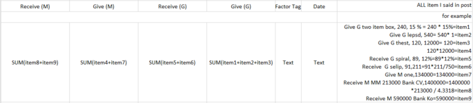
i have this worksheet that you see before, in first i said that belong to text, but that have information for main calculate, better say
in one cell i write information with this format : Give (+ Value) or Receive (-Value) ,G Or M, Text, Number, Percent or Thousands or Hundred (if Give and G and Percent: Percent that multiply to Number that written before this (if i not write anything in this part, multiply with 1), if Give and G and Thousands: Thousand multiply with number, if Receive and G and Percent: Percent multiply with number, if Receive and G and Hundred: Hundred multiply with number and then divide 750, for Give M that all this value sum and fill in specific columns that i say in below but for Receive M, if write MM after that calculate: Number multiply MM and divide 4.3318 if not write like Give M Calculate)
This fill in Column A
Columns B:C fill with Text without calculate
but in Column D
This fills with SUM of Gives and Back (+ Value) Calculates from G
in Column E
fills with SUM of Receive (- Value) Calculates from G
in Column F
fills with SUM of Gives (+ Value) Calculates from M
in Column G
fills with SUM of Receive (-Value) Calculates from M
and a point, i can't split information that belong one cell, because all of the info about a day and should write all info in one cell

 

[Unexpc]

#1
#2

or for this what things ordered that code can to find out...
please give an example thank you

 

[maabadi]

Numbers isn't No. Of Cases. They are case type. Then it is pissible you don't have case type 2 and 3. Then order is:
#1 ...... &
#4 ....... &
....
The ....... is your detail of each cases and can be everything based your case type.

 

[maabadi]

1# some

Yes. This is OK. Or
1- Some text then numbers and ... &
(If you don't have case type 2)
3- some text and numbers ... &
.....

 

[Unexpc]

1- Some text then numbers and ... &
(If you don't have case type 2)
3- some text and numbers ... &
.....

this separate not have order
but with type 1# that should write at first of any case, this is right? and can use instead of #, use ^ or anything?
please in this example file change to what your mind about this problem :Book Test P.xlsm

 

[Unexpc]

check this:Book Test P.xlsm

 

[maabadi]

Try this:
Book Test P.xlsm

 

[Unexpc]

Try this:
Book Test P.xlsm

i think i understood, instead of two character belong for each format, write number instead of this characters, am i right? if i say right, can use one symbol or character instead of numbers? for example for !# use ^ and for other formats use specific character
but still im not sure about, because probably i forgot write them in time of write factors, i don't know
the code can find different text and numbers together (i mean number or text different) for find differ in cases that have same formats?

 

[maabadi]

What is problem with this format I used?
Also you can add پرداخت or دریافت and any other words to case.
At this format, I search number between & symbol and - symbol to understand case type.
Then with more than one example for each case, calculated result for all of them belong to one case sum together.

You can change ( or add & remove cases) then see result when macro run.
I added worksheet change macro to worksheet at that file.

Yes. You can use symbols. But I need one symbol at the end of them to I can extract symbols. For example - I used at here.

 

[maabadi]

Also this is shorter version of Worksheet change event code for WORK sheet at my last updated file:

Private Sub Worksheet_Change(ByVal Target As Range)
Dim I As Long, J As Long, Lr1 As Long, Lr2 As Long, Cr As Long, CrR As String
Dim Lr3 As Long, Lr4 As Long, K As Long
Lr1 = Sheets("Dashboard").Range("I" & Rows.Count).End(xlUp).Row
Lr2 = Sheets("Dashboard").Range("N" & Rows.Count).End(xlUp).Row
Lr3 = Sheets("Work").Range("A" & Rows.Count).End(xlUp).Row
Lr4 = Sheets("Paper").Range("A" & Rows.Count).End(xlUp).Row

  If Intersect(Target, Range("A1:A" & Lr3)) Is Nothing Then Exit Sub
   On Error Resume Next
  Application.EnableEvents = False
    
  If Target.Interior.Color = 14277081 Then
  If Target.Value <> "" Then
  Range("A" & Target.Row & ":G" & Target.Row + Target.Value - 1).Insert Shift:=xlDown
  Target.Value = ""
  End If
  ElseIf Target.Interior.Color = 16777215 Then

Dim A As Double, B As Double, C As Double, D As Double, E As Double, F As Double, G As Double, H As Double
Dim I2 As String, J2 As Double, K2 As String, L As Double, M As Long, N As Long, O As Long, Lnum As Long
Dim T As String, P As Long, R As Long, S1 As Double, S2 As Double, W As Long, X As Long, Y As Long
Dim ii As Long, bb As Long, cc As Long, nn As Long, ee As Long, gg As Long, Lst As Long, pp As Long, rr As Long
T = Range("A" & Target.Row).Value
X = Len(T) - Len(Replace(T, "&", "")) + 1
For M = 1 To X
If M > 1 Then W = Application.WorksheetFunction.Find(Chr(1), Application.WorksheetFunction.Substitute(T, "&", Chr(1), M - 1))
  If M < X Then
   Y = Application.WorksheetFunction.Find(Chr(1), Application.WorksheetFunction.Substitute(T, "&", Chr(1), M))
  Else
   Y = Len(T)
  End If
   bb = Application.WorksheetFunction.Find(Chr(1), Application.WorksheetFunction.Substitute(T, "-", Chr(1), M))
   cc = Mid(T, W + 1, bb - W - 1)
   O = W + 4
For N = O To Y
If Mid(T, N, 1) = " " And IsNumeric(Mid(T, N + 1, 1)) Then P = N + 1
If IsNumeric(Mid(T, N, 1)) Or Mid(T, N, 1) = "." Or Mid(T, N, 1) = "/" Then pp = 1
If Not IsNumeric(Mid(T, N + 1, 1)) Or Mid(T, N + 1, 1) = "." Or Mid(T, N + 1, 1) = "." Then rr = 1
If pp = rr And pp > 0 Then R = N
If R >= P And P > 0 And Mid(T, N + 1, 1) = " " Or R = Len(T) Then
        If S1 = 0 Then
            S1 = Mid(Replace(T, "/", "."), P, R - P + 1)
            P = 0
            R = 0
        Else
            S2 = Mid(Replace(T, "/", "."), P, R - P + 1)
        End If
                If S2 <> S1 Then
                    Select Case cc
                            Case 1
                                If S2 > 0 Then A = A + Round(S1 * (1 + S2 / 100), 2)
                            Case 2
                                If S2 > 0 Then B = B + S1 * S2
                                If S2 > 0 Then J2 = J2 + S1
                            Case 3
                                If S2 > 0 Then C = C + Round(S1 * (1 + S2 / 100) * -1, 2)
                            Case 4
                                If S2 > 0 Then D = D + S1 * S2 * -1
                                If S2 > 0 Then L = L + S1 * -1
                            Case 5
                                E = E + S1 * 1
                                
                            Case 6
                                If S2 > 0 Then F = F + Round((S1 / S2) * 4.3318, 2)
                            Case 7
                                G = G + S1 * -1
                            Case 8
                                If S2 > 0 Then H = H + Round((S1 / S2) * -4.3318, 2)
                        
                    End Select
                    If S2 > 0 Or cc = 5 Or cc = 7 Then
                        S1 = 0
                        S2 = 0
                        P = 0
                        R = 0
                        GoTo Resum1
                    End If
                End If
End If

 pp = 0
 rr = 0
Next N
Resum1:
Next M
Range("D" & Target.Row).Formula = "=Round(" & A & "+" & J2 & "+" & F & ", 2)"
Range("E" & Target.Row).Formula = "=Round(" & C & "+" & L & "+" & H & ", 2)"
Range("F" & Target.Row).Formula = "=" & B & "+" & E
Range("G" & Target.Row).Formula = "=" & D & "+" & G

MsgBox "A1 = " & A & vbCr & "B1 = " & J2 & " // " & "B2 = " & B & vbCr & "C1 = " & C & vbCr & "D1 = " & L & " // " & "D2 = " & D _
& vbCr & "E1 = " & E & vbCr & "F1 = " & F & vbCr & "G1 = " & G & vbCr & "H1 = " & H

  
  
  End If
  For I = 3 To Lr1 - 1
   Cr = Application.WorksheetFunction.Match(Sheets("Dashboard").Range("I" & I).Value, Sheets("Work").Range("A1:A" & Lr3), 0)
   CrR = Range("A" & Cr).Address
     Sheets("Dashboard").Range("I" & I).Hyperlinks.Delete
     Sheets("Dashboard").Hyperlinks.Add Anchor:=Sheets("Dashboard").Range("I" & I), Address:="", SubAddress:="'" & Sheets("Work").Name & "'!" & CrR, TextToDisplay:=Sheets("Dashboard").Range("I" & I).Value
     With Sheets("Dashboard").Range("I" & I)
                .Font.Underline = xlUnderlineStyleNone
                .Font.ColorIndex = xlColorIndexAutomatic
                .Font.Name = "Microsoft Parsi"
                .Font.Size = 14
                .HorizontalAlignment = xlCenter
                .VerticalAlignment = xlCenter
     End With
  Next I
  Application.EnableEvents = True
End Sub

 

[Unexpc]

At this format, I search number between & symbol and - symbol to understand case type.

yes you use same number before - for same formats, i say probably i forgot write same number for same formats, if like a list number (1-,2-,3-,4-,5-...) for each case i write, this is very good, but for same format write same number, this probably make a mistake for me
i mean this is good like you say before?(am i right?)
1#.........
2#.........
3#.........
4#.........
5#.........
6#.........
instead of # other symbol or that # is ok, but i test with - in your example file and that can't calculate (please see photo)

Also you can add پرداخت or دریافت and any other words to case.

yes i understood and this is very good