Condition formatting for tolerancing

[HighSpeed]

I have found a lot of info about using conditional formatting to indicate tolerances but not quite what I'm looking for. I don't know if this is even possible.

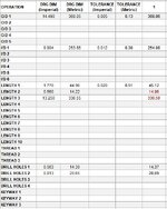
I am modifying a dimensional checking sheet to show if a measured dimension is out of tolerance, IF there is a tolerance for that particular dimension. We do get drawings both in imperial and metric but we only use metric equipment, so I also have the converted dim next to the drawing dim. See attached pic.

I have a column (B8:B38) which has the nominal dimension shown. Next to that, I have another column which will be a tolerance if a tolerance is required for that particular nominal dim, which I will enter as a positive value to keep it simple. I have conditional formatting working fine when there is a tolerance by having 2 rules - if value is less than nominal, then colour text red, and if value is more than nominal plus tolerance, then colour text red. This is where it goes wrong... if there is no tolerance, I don't want to colour the text. If I have no number in the tolerance cell and the measured value is less than the nominal value, it is colouring the text. It will not colour the text if the measured value is above the nominal dim.

I'm thinking something along the lines of "if tolerance cell has a number, then use conditional formatting, otherwise do not use conditional formatting". I just don't know how to go about that, or if it is even possible to do with conditional formatting. Can anyone help please?

 

[etaf]

=AND( Cell <> "", Cell = tolerance )

as a conditional formatting rule

so just add the AND( Cell <> "" , your existing formula)

BUT

Note: Images are difficult to see , and also requires that I input all the data myself, which is very time consuming.

A SMALL sample spreadsheet, around 10-20 rows, would help a lot here, with all sensitive data removed, and expected results mocked up and manually entered, with a few notes of explanation.

MrExcel has a tool called “XL2BB” that lets you post samples of your data and will allow us to copy/paste your sample data into our Excel spreadsheets, saving a lot of time.

XL2BB - Excel Range to BBCode

Excel 'mini-sheet' in messages - XL2BB Although experts prefer to read your description and question instead of working in your actual file to solve your problem, there are times that it is difficult to explain an issue without providing actual...

www.mrexcel.com

You can also test to see if it works ok, in the "Test Here" forum.

Test Here

Use this forum to test your signature, learn bbcode, smilies, XL2BB, etc. Threads in this forum are automatically deleted after no replies for seven (7) days

www.mrexcel.com

OR if you cannot get XL2BB to work, or have restrictions on your PC , then put the sample spreadsheet onto a share
I only tend to goto OneDrive, Dropbox or google docs , as I'm never certain of other random share sites and possible virus.
Please make sure you have a representative data sample and also that the data has been desensitised, remember this site is open to anyone with internet access to see - so any sensitive / personal data should be removed

 

[HighSpeed]

=AND( Cell <> "", Cell = tolerance )

as a conditional formatting rule

so just add the AND( Cell <> "" , your existing formula)

BUT

Note: Images are difficult to see , and also requires that I input all the data myself, which is very time consuming.

A SMALL sample spreadsheet, around 10-20 rows, would help a lot here, with all sensitive data removed, and expected results mocked up and manually entered, with a few notes of explanation.

MrExcel has a tool called “XL2BB” that lets you post samples of your data and will allow us to copy/paste your sample data into our Excel spreadsheets, saving a lot of time.

XL2BB - Excel Range to BBCode

Excel 'mini-sheet' in messages - XL2BB Although experts prefer to read your description and question instead of working in your actual file to solve your problem, there are times that it is difficult to explain an issue without providing actual...

www.mrexcel.com

You can also test to see if it works ok, in the "Test Here" forum.

Test Here

Use this forum to test your signature, learn bbcode, smilies, XL2BB, etc. Threads in this forum are automatically deleted after no replies for seven (7) days

www.mrexcel.com

OR if you cannot get XL2BB to work, or have restrictions on your PC , then put the sample spreadsheet onto a share
I only tend to goto OneDrive, Dropbox or google docs , as I'm never certain of other random share sites and possible virus.
Please make sure you have a representative data sample and also that the data has been desensitised, remember this site is open to anyone with internet access to see - so any sensitive / personal data should be removed

Thanks Wayne. I've got it installed but cannot get XL2BB to work... there is nothing proprietary in the sheet anyway but for simplicity I've uploaded the appropriate section to a sample sheet - Sample Inspection.xlsx

I currently use the "Cell value < $C2" and "Cell value > $C2+$E2" rules for the conditional formatting. How would I express that in formula instead, in order to include the AND argument? Can I just use literally "Cell Value"? Apologies, I don't use formulas enough to wrap my head around this.

 

[Sulprobil]

Hello,

A general approach: apply the conditional format formula:

=Cell<>MEDIAN(Cell,Cell-Lower_Tolerance,Cell+Upper_Tolerance)

If a cell has no tolerance boundaries, set both lower and upper tolerance to 1e200.

Regards,
Bernd

 

[Sulprobil]

...

=Cell<>MEDIAN(Cell,Cell-Lower_Tolerance,Cell+Upper_Tolerance)

...

Of course the last two "Cell" references need to refer to another reference cell or you omit them to make the tolerance boundaries absolute one's.

 

[etaf]

you have 2 rules
cell value < $C2
and
Cell value > $C2+$E2

and that applies to F2:G32

so we can change that to add a formula

=AND ( F2 < $C2 , $C2<>"" )

But your existing rules are comparing the value in column C to F & G
is that what you want to be comparing ?

just to help others - i have used XL2BB here to show the linked file - NOTHING Changed

[

Sample Inspection.xlsx
	A	B	C	D	E	F	G
1	OPERATION	DRG DIM (Imperial)	DRG DIM (Metric)	TOLERANCE (Imperial)	TOLERANCE (Metric)	1	2
2	O/D 1	14.490	368.05	0.005	0.13	368.30
3	O/D 2
4	O/D 3
5	O/D 4
6	O/D 5
7	I/D 1	9.994	253.85	0.012	0.30	253.89
8	I/D 2
9	I/D 3
10	I/D 4
11	I/D 5
12	I/D 6
13	LENGTH 1	1.770	44.96	0.020	0.51	44.98
14	LENGTH 2	0.560	14.22			14.20
15	LENGTH 3	13.250	336.55			336.52
16	LENGTH 4
17	LENGTH 5
18	LENGTH 6
19	LENGTH 7
20	LENGTH 8
21	LENGTH 9
22	LENGTH 10
23	THREAD 1
24	THREAD 2
25	THREAD 3
26	DRILL HOLES 1	0.563	14.30			14.30
27	DRILL HOLES 2	0.813	20.65			20.68
28	DRILL HOLES 3
29	DRILL HOLES 4
30	KEYWAY 1
31	KEYWAY 2
32	KEYWAY 3
Sheet1

Cell Formulas
Range	Formula
C2:C22,E2:E32,C26:C32	C2	=IF(ISNUMBER(B2),B2*25.4,"")

Cells with Conditional Formatting
Cell	Condition		Cell Format	Stop If True
B26:B27	Expression	=MOD(ROW(),2)=0	text	YES
B2:B7	Expression	=MOD(ROW(),2)=0	text	YES
B8:B15	Expression	=MOD(ROW(),2)=0	text	YES
F2:G32	Cell Value	<$C2	text	NO
F2:G32	Cell Value	>$C2+$E2	text	NO
A28:C32,A23:B25,A16:C22,A1:G1,C2:G2,A2:A15,C3:C15,A26:A27,C26:C27,D3:G32	Expression	=MOD(ROW(),2)=0	text	YES

 

[HighSpeed]

Really appreciate the ideas. I'm so out of touch on this stuff... I'm somewhat confused about what I should actually have in the formula bar. Do I delete the two rules I have in there now and create a new formula rule " =AND(F2<$C2,$C2<>"") " Having tried just that and not seeing any difference, I'm guessing I'm missing something?? Please remember what some people think of as a given, will not necessarily occur to someone else. I know full well I'm out of my depth, hence why I'm asking on here. When I started this, I was trying to work out if there is a way to add an IF(ISNUMBER) argument to conditional formatting. If there is no number in the tolerance column, then don't format the resulting cell(s). It seems simple to me but I havent got the faintest idea how to APPLY that to conditional formatting.

Having the two rules that are there now works fine when there is a tolerance. It might be a "messy" way to do it but the spreadsheet is simple and a little bit of bloat is not an issue.

Columns C & E are there to convert imperial measurements to metric. Columns F to O are the physically checked dimensions from the part and need to be compared to the values in C & E, changing colour if it is out of tolerance, but ONLY if there is a tolerance for that line.

As far as the XL2BB goes, I installed it but only had 2 buttons to pick from and both were greyed out. Hence why I said I couldnt get it to work. It threw up a message saying something about disabling macros and went into some kind of protected mode. I'm rather paranoid about giving access to my computer for anything I dont know well and using a dropbox linked file is easy enough so I left it at that.

 

[etaf]

Please remember what some people think of as a given, will not necessarily occur to someone else.

I understand and usually will try not to make too many assumptions - but may have here

I have looked at the dropbox link and tried to understand the spreadsheet from your text - but that is not quite making sense to me

looking at the columns A to G in your spreadsheet

OPERATION

DRG DIM (Imperial)

DRG DIM (Metric)

TOLERANCE (Imperial)

TOLERANCE (Metric)

1

2

Column D and E are labelled Tolerance

Columns C & E are there to convert imperial measurements to metric.

However you mention C & E - convert NOT tolerance

Columns F to O are the physically checked dimensions from the part and need to be compared to the values in C & E, changing colour if it is out of tolerance,

F has a 1 as label and G has a 2
You say this would go from F to O , as checked dimensions
What do those 10 columns check ???

but ONLY if there is a tolerance for that line.

I would Assume - and not doing that - so asking here
That the tolerance is in D & E

So if D or E is blan , then do not highlight column F to O
but which tolerance are we looking at for each of those columns

Is it that BOTH D and E will be blank - then do not conditional format

you have 2 rules which make the text RED

as mentioned in previous post

you have 2 rules
cell value < $C2
and
Cell value > $C2+$E2

and that applies to F2:G32

=AND(F2<$C2,$D2<>"",$E2<>"",F2<>"")
=AND(F2 > $C2+$E2 ,$D2<>"",$E2<>"",F2<>"")

so the only cell that will highlight is
F2
and NOT
row 14 or 15 or 26 - as those rows have NO entry in columns D & E

or have i completely misunderstood -

I have a link here with those formulas entered - and i have formatted with a FILL as well as the text - that can be changed - but wanted a good visual indication

Dropbox - File Deleted - Simplify your life

www.dropbox.com

Sample Inspection-ETAF.xlsx
	A	B	C	D	E	F	G	H	I	J	K	L	M	N	O	P	Q	R	S	T
1	OPERATION	DRG DIM (Imperial)	DRG DIM (Metric)	TOLERANCE (Imperial)	TOLERANCE (Metric)	1	2
2	O/D 1	14.490	368.05	0.005	0.13	368.30				Columns C & E are there to convert imperial measurements to metric. Columns F to O are the physically checked dimensions from the part and need to be compared to the values in C & E, changing colour if it is out of tolerance, but ONLY if there is a tolerance for that line.
3	O/D 2
4	O/D 3
5	O/D 4
6	O/D 5
7	I/D 1	9.994	253.85	0.012	0.30	253.89
8	I/D 2
9	I/D 3
10	I/D 4
11	I/D 5
12	I/D 6
13	LENGTH 1	1.770	44.96	0.020	0.51	44.98
14	LENGTH 2	0.560	14.22			14.20
15	LENGTH 3	13.250	336.55			336.52
16	LENGTH 4
17	LENGTH 5
18	LENGTH 6
19	LENGTH 7
20	LENGTH 8
21	LENGTH 9
22	LENGTH 10
23	THREAD 1
24	THREAD 2
25	THREAD 3
26	DRILL HOLES 1	0.563	14.30			14.30
27	DRILL HOLES 2	0.813	20.65			20.68
28	DRILL HOLES 3
29	DRILL HOLES 4
30	KEYWAY 1
31	KEYWAY 2
32	KEYWAY 3
Sheet1

Cell Formulas
Range	Formula
C2:C22,E2:E32,C26:C32	C2	=IF(ISNUMBER(B2),B2*25.4,"")

Cells with Conditional Formatting
Cell	Condition		Cell Format	Stop If True
F2:G33	Expression	=AND(F2 > $C2+$E2,$D2<>"",$E2<>"",F2<>"")	text	NO
F2:G33	Expression	=AND(F2<$C2,$D2<>"",$E2<>"",F2<>"")	text	NO
B26:B27	Expression	=MOD(ROW(),2)=0	text	YES
B2:B7	Expression	=MOD(ROW(),2)=0	text	YES
B8:B15	Expression	=MOD(ROW(),2)=0	text	YES

 

[HighSpeed]

Reading my own comments, I may be guilty of doing the same thing! Sorry... So when we make certain parts from a drawing, the parts need to be checked off against the manufacturing drawing. Generally for us, that will be 10 or less parts... those checked dimensions will be entered into columns F - O. For simplicity, assume I'm only checking one part and disregard columns G-O completely - treat column F as the only column that needs conditional formatting. More often than not for whatever reason, one particular customer gives us drawings with imperial dimensions. As all of our machines and measuring gear are all metric, I needed a simple way to convert the imperial dims to metric so I can check them without having to use a calculator every time. The drawing dimension is entered in column B and column C will simply convert that imperial dimension to metric with =IF(ISNUMBER(B2),B2*25.4,""). In the same way, if there is a critical part that requires a tolerance, then I will put it in the tolerance column. The imperial columns for this exercise are basically irrelevant to the conditional formatting - the converted metric data is what I'm actually checking, so if it makes it easier, columns B & D can just be hidden.

That file is exactly what I'm trying to do. Legend! I just couldn't get my head around the way it had to be entered as a formula. Apologies for my lack of clarity but you have hit the nail on the head anyway.

 

[etaf]

you are welcome