Ctrl F, export results

[ellison]

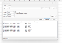
Hi, I'm wondering if there is a way of exporting the results of a Ctrl Find?

I've seen that you can select them all and copy them, but only if the selected cells are next to each other. (But that doesn't happen very often for us!).

(The other challenge we have is that we'd like to use this on different files & they'll often have different headers, sheet names etc

Ctrl-Find-Export-Results-01.xlsx
	A	B	C	D
1	Row	Col-B	Col-C	Col-C
2	2	alpha	alpha 9
3	3	beta
4	4	charlie	charlie 6
5	5	delta	delta	14
6	6	echo	echo 5
7	7	foxtrot	foxtrot 1	12
8	8
9	9	golf	golf 4
10	10	hotel	hotel 4
Sheet1

Thanks for any help you could provide!

 

[duggie33]

Hi ellison,

You can use FILTER on each column like below...

Book1
	A	B	C	D	E	F	G	H	I	J
1	Row	Col-B	Col-C	Col-C				alpha	alpha 9
2	2	alpha	alpha 9					beta	charlie 6
3	3	beta						charlie	delta
4	4	charlie	charlie 6					delta
5	5	delta	delta	14
6	6	echo	echo 5
7	7	foxtrot	foxtrot 1	12
8	8
9	9	golf	golf 4
10	10	hotel	hotel 4
Sheet1

Cell Formulas
Range	Formula
G1,J1,I1:I3,H1:H4	G1	=FILTER(A$1:A$10,ISNUMBER(SEARCH("a",A$1:A$10,1)),"")

I tried to adapt it to BYCOL and had errors. With a little searching, I discovered @Xlambda has a CBYCOL that overcomes the errors and allows a single formula to return all the results. I have not spent enough time to figure out how it works yet. I may try to figure out how to take the CBYCOL results, FILTER out blanks, and VSTACK the results, but that would require time I do not have at the moment.

It is not clear how you would like the results formatted, so maybe this will be the starting point.

Hope that helps,

Doug

 

[ellison]

Hi, wow that looks really promising!

Ideally the results would be pasted into 1 column (where we get to enter the cell address for the starting point eg H1), or even better, be able to paste them into notepad..

Either would be great, whatever would be easier...

With thanks

 

[duggie33]

To use this you will have to add the LAMBDA function, CBYCOL, created by @Xlambda. To do that, go to the Name Manager and add a new name called CBYCOL and then put the following in the "Refers to:" box:

=LAMBDA(ar,fn,LET(a,IF(ar="","",ar),w,--(ROWS(a)=1),r,REDUCE(0,SEQUENCE(COLUMNS(a)),LAMBDA(v,i,HSTACK(v,fn(INDEX(a,w,i))))),DROP(IFNA(r,""),,1)))

Book1
	A	B	C	D	E	F	G
1	Row	Col-B	Col-C	Col-C		t	beta
2	2	alpha	alpha 9				delta
3	3	beta					foxtrot
4	4	charlie	charlie 6				hotel
5	5	delta	delta	14			delta
6	6	echo	echo 5				foxtrot 1
7	7	foxtrot	foxtrot 1	12			hotel 4
8	8
9	9	golf	golf 4
10	10	hotel	hotel 4
Sheet1

Cell Formulas
Range	Formula
G1:G7	G1	=LET(arr,A1:D10,findthis,F1,filtrng,CBYCOL(arr,LAMBDA(rngcol,FILTER(rngcol,ISNUMBER(SEARCH(findthis,rngcol,1)),""))),singlecol,TOCOL(filtrng,1,TRUE),FILTER(singlecol,singlecol<>""))
Dynamic array formulas.

Hope it works for you,

Doug

 

[ellison]

Wow this looks great-…. I need to clear some time to try and get this working.
I’ll report back in and let you know how I get on.
(This may take a Luddite like me a bit of time to get my head around!)

 

[ellison]

Sorry - haven't forgotten this, just bashing away at trying to get it working!

 

[ellison]

Hi, please find some more details re: the CBYCOL. And solution marked up (apologies for delay!).

In the main menu ribbon / Formulas / Name Manager / In Name: CBYCOL / In Refers to: =LAMBDA(ar,fn,LET(a,IF(ar="","",ar),w,--(ROWS(a)=1),r,REDUCE(0,SEQUENCE(COLUMNS(a)),LAMBDA(v,i,HSTACK(v,fn(INDEX(a,w,i))))),DROP(IFNA(r,""),,1)))

In Cell F1, insert what you're searching for

In Cell G1: enter as dynamic array: =LET(arr,A1:D10,findthis,F1,filtrng,CBYCOL(arr,LAMBDA(rngcol,FILTER(rngcol,ISNUMBER(SEARCH(findthis,rngcol,1)),""))),singlecol,TOCOL(filtrng,1,TRUE),FILTER(singlecol,singlecol<>""))
NB Ctrl + Shift + Enter

Hope this helps

 

[ellison]

Sorry duggie33, I've unticked the solution....

On reflection, whilst the CBYCOL is a really useful tool, it doesn't quite tick the boxes of what we were trying to achieve.

HUGE Positive: it lists the contents of cells containing whatever string is searched for
BUT
Negative-01: the cell addresses aren't included
Negative-02: it doesn't search formulas (or the results of formulas)

What we were originally looking to do was be able to (similar to exporting the results of (Ctrl+F / Find-All):

- list the cell addresses & contents
- containing whichever string
- in either the formula OR the values
(wouldn't ever need to use the "entire cell contents" or "matching case")

Would anybody have any pointers?

Huge thanks for reading this far ...

 

[Georgiboy]

You can give the below sub a try, when run, it will ask you first for the search string, second for the cell to start placing the results:

Sub FindLoop()
    Dim addVar() As String, valVar() As String, x As Long
    Dim rngFA As String, outIB As Range
    Dim rng As Range, fRng As Range
    
    Set rng = ActiveSheet.UsedRange
    Set fRng = rng.Find(InputBox("Value to find", "Find what?"), , , xlPart)
    
    If Not fRng Is Nothing Then
        rngFA = fRng.Address
        Do
            ReDim Preserve addVar(x): addVar(x) = fRng.Address(, , , 1)
            ReDim Preserve valVar(x): valVar(x) = fRng.Value
            x = x + 1
            Set fRng = rng.FindNext(fRng)
        Loop Until fRng Is Nothing Or fRng.Address = rngFA
    End If
    
    Set outIB = Application.InputBox("Select range", Type:=8)
    
    outIB.Resize(UBound(addVar) + 1, 1) = Application.Transpose(addVar)
    outIB.Offset(, 1).Resize(UBound(valVar) + 1, 1) = Application.Transpose(valVar)
End Sub

 

[ellison]

Crumbs that is absolutely brilliant, HUGE thanks!

I've got a couple of questions..... just wondering if:

1. Is it possible to limit the searches to either searching in "values" or "formulas" [at the moment the code is searching "both"]

2. Also, is it possible in the results to display either "value" or "formula" [at the moment, it's showing the values]

So raw info is still in A1:E10
- any grey cells in the raw data are formulas

Code Output is in I2:J5

(The other bits are helper columns which I've added in manually - to confirm: they aren't needed, they're hopefully just there to help explain a little bit better!)

Ctrl-Find-Export-Results-03.xlsm
	A	B	C	D	E	F	G	H	I	J	K	L	M
1	Row	Col-B	Col-C	Col-D: formulas	Col-E: formula		Results of search for "the digit six":		Code-Output-A	Code-Output-B	Help-01: Address	Help-02: Formula	Help-03: Value
2	2	alpha	alpha 9	2	echo		- plus added in some headers		[Ctrl-Find-Export-Results-03.xlsm]Sheet1'!$E$2	echo	E2	=+B6	echo
3	3	beta		4			- none of the headers or helper columnss are actually needed		[Ctrl-Find-Export-Results-03.xlsm]Sheet1'!$C$4	charlie 6	C4	n/a	charlie 6
4	4	charlie	charlie 6	6			- (...they're only to help explain!)		[Ctrl-Find-Export-Results-03.xlsm]Sheet1'!$A$6	6	A6	n/a	6
5	5	delta	delta	8					[Ctrl-Find-Export-Results-03.xlsm]Sheet1'!$D$7	12	D7	=+2*6	21
6	6	echo	echo 5	10
7	7	foxtrot	foxtrot 1	12
8	8
9	9	golf	golf 4
10	10	hotel	hotel 4
Sheet1

Cell Formulas
Range	Formula
E2	E2	=+B6
D2	D2	=1*2
D3	D3	=2*2
D4	D4	=2*3
D5	D5	=2*4
D6	D6	=2*5
D7	D7	=2*6

Huge thanks (again!!!)