Daily pickups.

Learning 101

New Member
Joined
Feb 1, 2021
Messages
6
Office Version
  1. 365
Platform
  1. Windows
I have 6 columns.
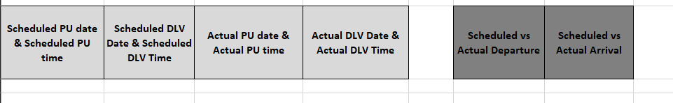
Column A = Scheduled PU date & Scheduled PU time
Column B = Scheduled DLV Date & Scheduled DLV Time
Column C = Actual PU date & Actual PU time
Column D = Actual DLV Date & Actual DLV Time
Column F = Scheduled vs Actual Departure
Column G =Scheduled vs Actual Arrival

If the shipment was picked up early, column F cells have to turn blue and say "Early by "hh:mm"
If the shipment was picked up on time, column F cells have to turn green and say "on time"
If the shipment was picked up late, column F cells have to turn red and say "LATE by "hh:mm"

If the shipment was delivered early, column G cells have to turn blue and say "Early by "hh:mm"
If the shipment was delivered on time, column G cells have to turn green and say "on time"
If the shipment was delivered late, column G cells have to turn red and say "LATE by "hh:mm"

1612206865167.png
 

Attachments

  • 1612206831608.png
    1612206831608.png
    14 KB · Views: 11

Excel Facts

Show numbers in thousands?
Use a custom number format of #,##0,K. Each comma after the final 0 will divide the displayed number by another thousand
=IF((MID(f2,1,2)&":"&MID(f2,3,2))*1-(MID(g2,1,2)&":"&MID(g2,3,2))*1<0,"EARLY",IF((MID(g2,1,2)&":"&MID(f2,3,2))*1-(MID(g2,1,2)&":"&MID(g2,3,2))*1>0.0208333333333333,"LATE","ON TIME"))
 
Upvote 0
Welcome to the board!

The basic formula you're asking for might be something like
Excel Formula:
=IF($A2>$C2,"Early by","LATE by")&" "&TEXT(ABS($C2-$A2),"[hh]:mm")

However, if you stick with that it's quite impossible to do any further calculations on the accuracy: Sooner or later you're going to want to know the average accuracy and see how that changes over time. To be able to do that you should split that in two columns and if you do that, you want to get rid of that TEXT-formula: The ABS($C2-$A2) is enough in your other column and if you format your time column with [hh]:mm time format, you're going to see the times in hours and minutes even if they're past 24 hours. Unfortunately Excel is having problems displaying negative times so you're going to have to keep the ABS-bit if you want to show the hours & minutes on row each row.

Also, as you wanted to see some shipments being picked up or delivered in time you're going to need to use some kind of a buffer in your calculations:
Excel Formula:
=IF($A2-Buffer>$C2,"Early",IF($A2+Buffer<$C2,"Late","On Time"))

For the conditional formatting (cell color change) you might want to use something like
Excel Formula:
=LEFT(F2,4)="Late"
As Excel time values can not be negative you're going to have to compare the text values alone.
 
Upvote 0
Misca, you're a lifesaver!! Thank you!

Just one question, for the below formula. Either late or early, whatever it is, it only shows up as LATE. Can you fix that and also add "ON TIME" if the value is 0.

=IF($A2>$C2,"Early by","LATE by")&" "&TEXT(ABS($C2-$A2),"[hh]:mm")
 
Upvote 0
Replace the first bit with my second formula. It references the buffers which you're going to need if your times are actual time stamps: It's very unlikely you're going to get the times to match to a fraction of a second.

The buffer in my formula is a named range: Select a cell and type Buffer to the address/name box (left of the formula bar). Your selection is now known as Buffer and you can use that in all your formulas when you want to reference that range. If you type 30 minutes to your named range the formula returns "On time" as long as the time difference from the scheduled time is within the 30 minutes.
 
Upvote 0
Thank you! Misca, I think everything is set. the only issue I'm having now is that there's only "On Time:" that's showing up. Any time difference, only one thing is showing up.


=IF(h4-Buffer1>j4,"Early",IF(h4+Buffer1<j4,"Late","On Time"))&" "&TEXT(ABS(j4-h4),"[hh]:mm")

Buffer1 is J4

1612462096381.png
1612462120349.png
 
Upvote 0
Try this:
Excel Formula:
=IF(A4-Buffer1>C4,"Early",IF(A4+Buffer1<C4,"Late","On Time"))&" "&TEXT(ABS(C4-A4),"[hh]:mm")
 
Upvote 0
that's the same exact formula I posted above. Instead of showing early, on time, or late respectively, it only shows "Ontime" for all calculations. PLEASE HELP!
 
Upvote 0
The green cell is my Buffer:
Boogie.xlsx
ABCDEFG
1Buffer:
20:30
3
4ScheduledActualScheduled vs ActualShipmentOffset
504.02.2021 10:0004.02.2021 10:29On Time 00:29On Time00:29
604.02.2021 10:0009.02.2021 13:45Late 123:45Late123:45
704.02.2021 10:0004.02.2021 9:29Early 00:31Early00:31
8
Sheet1
Cell Formulas
RangeFormula
F5:F7F5=IF(A5-Buffer>B5,"Early",IF(A5+Buffer<B5,"Late","On Time"))
G5:G7G5=ABS(B5-A5)
D5:D7D5=IF(A5-Buffer>B5,"Early",IF(A5+Buffer<B5,"Late","On Time"))&" "&TEXT(ABS(B5-A5),"[tt]:mm")
Named Ranges
NameRefers ToCells
Buffer=Sheet1!$D$2D5:D7, F5:F7
Cells with Conditional Formatting
CellConditionCell FormatStop If True
D5:D7Expression=LEFT($D5;5)="Early"textNO
D5:D7Expression=LEFT($D5;4)="Late"textNO
 
Upvote 0
If your formula always returns "On Time" make sure your buffer is in hours not in days.
 
Upvote 0

Forum statistics

Threads
1,215,491
Messages
6,125,108
Members
449,205
Latest member
ralemanygarcia

We've detected that you are using an adblocker.

We have a great community of people providing Excel help here, but the hosting costs are enormous. You can help keep this site running by allowing ads on MrExcel.com.
Allow Ads at MrExcel

Which adblocker are you using?

Disable AdBlock

Follow these easy steps to disable AdBlock

1)Click on the icon in the browser’s toolbar.
2)Click on the icon in the browser’s toolbar.
2)Click on the "Pause on this site" option.
Go back

Disable AdBlock Plus

Follow these easy steps to disable AdBlock Plus

1)Click on the icon in the browser’s toolbar.
2)Click on the toggle to disable it for "mrexcel.com".
Go back

Disable uBlock Origin

Follow these easy steps to disable uBlock Origin

1)Click on the icon in the browser’s toolbar.
2)Click on the "Power" button.
3)Click on the "Refresh" button.
Go back

Disable uBlock

Follow these easy steps to disable uBlock

1)Click on the icon in the browser’s toolbar.
2)Click on the "Power" button.
3)Click on the "Refresh" button.
Go back
Back
Top