Display the Slicer Selction in Excel Cells

[Dheepak]

Hi,

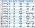
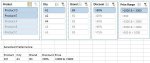
I have a data set and converted to table (not pivot table/chart - done via Ctrl+T). There are total 5 filters i have kept to view the details. Slicer 1 has products, Slicer 2 has city, Slicer 3 has brand and so on. If i select Product A,City A, and Brand A, i need to get cell A1 updated with the selected values of prodcut, city and brand. Can someone guide on how to achieve this.

Regards,
Dheepak

 

[PCL]

Can you give more details with picture, data examples ...?

 

[Dheepak]

Hi, Please find the attached details and kindly let me know in case of additional details. Need to get updated with ";" if there are multi values selected. Thank you

 

[PCL]

I'm not sure to get it right.
With the first slicer you make a selection: Is shown Items corresponding to this selection
Then with the second one you do another selection and is displayed Items corresponding to selection 1 and 2
And so one ...!
What the issue for you

 

[Dheepak]

Those are the ones i typed manually for example purpose. So the columns should get updated and needs to changed accordingly based on the selection from the slicer. Like if 5 check box are there, i can code it like once it selected update the cell with that value and once its de-selected delete the value. If two check box selected, it should updated with Check box 1; Check box 2. In similarly way, looking for the options to perform it with slicer with table as a source.

 

[PCL]

Are your slicer linked to the table?
If not , slect the table, select Insert > Slicer

 

[Dheepak]

Yes, its linked to the table. how i can able to display it in one column the selected values instead of getting my complete table filtered is the issue i'm facing. As Source data with some additional details will in other sheet. Slicers will be in selection page. So based on the slicer selection, if there are three rows in the table with product A two entries and product B one entries, i would like to get it displayed in product cell with value as "product A; product B"

 

[PCL]

As far as I have understood, it looks like you want a table for each field with no link with others and a slicer for each field acting only on one field.
It seems not possible ... tables in the same sheet are linked and therefore a selection on a table has some consequences on the others.

If it is the issue you are running into, a way to avoid such problem could be to use Pivot Table:
A Pivot Table for each field
Then in the Pivot Table you can make selection independantly of others fields ...!

 

[Dheepak]

Thank you so much for your help. Is it possible that once applied filter, i can join the text for the filtered one instead of complete column.

Eg: I have list of products A to F. If i applied the slicer product A & product B, the table will get filtered with all the records which are having product A & B. However, i need only value of product A & product B and it should be updated with the separation (semicolon).

I have tried =CONCATENATE(A1,";",A2,";",A3,";",A4,";",A5,";",A6,";",A7,";",A8,";",A9,";",A10) but here unable to check the unique value and its not pulling the filtered columns. Instead all the products from A1 to A10 its getting updated while only Cell A2, A4 are having product A and A8,A9 are having product B.

Could you please guide on how to achieve this.. Thank you once again..