Dynamic Data Point Markers in a graph/chart

[SerenityNetworks]

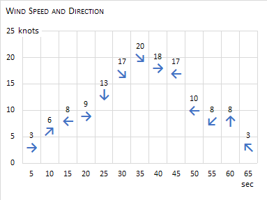
I'm plotting temperature, wind speed, and wind direction by time. For the wind direction, I'd like to display an arrow or icon that matches the wind direction. For example, if the wind is blowing to the east then I'd like a right pointing arrow on the chart. I'd like to do this for the 16 principle points of the compass. Is this possible in Excel using standard functionality? If so, will someone point me to instructions or step me through how to do it?

Thanks in advance,
Andrew

 

[Jon Peltier]

It's "standard" functionality but tricky and not automatic. Here's what you need to do.

1. Make yourself the 16 arrows you need by drawing arrow autoshapes in the worksheet.

2. Plot the points, using any old marker.

3. For each point:

A. Copy the arrow you need based on the direction it represents.

B. Select the data point (two single clicks: the first click selects the series of points, the second click selects the individual point).

C. Paste using Ctrl+V.

If you have a lot of these, it can be automated with VBA. I wrote a tutorial a decade ago, but I can't seem to locate it. If you're interested, maybe I can reproduce that old topic.

 

[thisoldman]

Not exactly as requested. I think you wanted something close to this: http://robslink.com/SAS/democd11/isabel2.htm

I came up with this:

I can't give sixteen points on the wind direction, but I came up with eight.

sec	knots	knots_2	Direction	Marker
5	3	3	5	↖
10	6	6	6	↗
15	8	8	1	←
20	9	9	3	→
25	13	13	4	↓
30	17	17	7	↘
35	20	20	7	↘
40	18	18	3	→
45	17	17	1	←
50	10	10	1	←
55	8	8	8	↙
60	8	8	2	↑
65	3	3	5	↖

<tbody>
</tbody>

I converted the wind direction to an integer between 1 and 8. The eight arrows come from Insert > Symbols > Symbol > Subset:Arrows. The formula in the rightmost column is:

=CHOOSE(E3,"←","↑","→","↓","↖","↗","↘","↙")

I chose a line graph but a scatter plot works as well. I selected the three leftmost columns and inserted a chart, both series with markers.

For one series I added Data Labels: Above to show the wind speed.

This method only works in Excel 2013 and later. For the second series, I added Data Labels centered on the point markers. I chose Label Options > Label Contains: Value From Cells. In the range selection box that popped up, I selected the cells with the arrow symbols. The chart is 3 x 4 inches, I chose 14 pt Calibri Bold as the font face, with a blue color. The font choice is important:

I then formatted the two series to have no lines and no markers.

 

[thisoldman]

The actual formula for the CHOOSE function should probably go around the compass rose:

=CHOOSE(E3,"←","↖","↑","↗","→","↘","↓","↙")

 

[SerenityNetworks]

Thank you Jon and ThisOldMan. I'm trying to stay away from VBA in this project, if at all possible, so I'm going to give ThisOldMan's solution a whirl.

Yes, you are exactly right, something like the hurricane graph would be ideal. But I'm willing to go with something like the solution you presented. Using the eight points will be sufficient for now (and maybe forever). If I want more, I might look into creating a custom font that is stored with the workbook. Thank you for the detailed instructions. Following those steps will make the implementation quite easy. I don't think I would have ever thought of using font symbols for the display. Now that's what I call creative.

Thanks again,
Andrew