Dynamic worksheet look up - index match 2-way look up

[windb]

Hi there,

I have an index match match 2-way look up, which returns data based on another tab. (The index match does a vertical look up and then a horizontal one). The formula works fine, but I would like to introduce a variable into the formula to so it looks up the 'correct' tab, corresponding with the value in column A. I'm not familiar with the Indirect formula, but have tried giving this a go with no success. Is this possible?

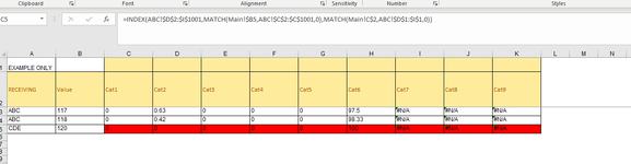
The formula needs to allow for the fact that I may have up to 20 or so receiving IDs/ tabs. The range for all tabs will the same, albeit the detail contained within the tabs will be different. Ordinarily, I would just use an IF statement, e.g. IF ABC, then look up the ABC tab, etc but this doesn't feel very efficient in instances where there will be multiple scenarios.

I have attached an image which shows the formula in red, where ideally I would like this to look up tab "CDE" automatically.

Many thanks - appreciate any help in advance!

 

[etaf]

i have made up an example - not following the image as difficult to see and match

i can change your formula BUT post it in the text of a post so i can copy

so the formula
=INDEX(Sheet2!B2:E5,MATCH(Sheet1!A3,Sheet2!A2:A5,0),MATCH(Sheet1!B3,Sheet2!B1:E1))

is replaced by
=INDEX(INDIRECT("'"&C6&"'!B2:E5"),MATCH(Sheet1!A6,INDIRECT("'"&C6&"'!A2:A5"),0),MATCH(Sheet1!B6,INDIRECT("'"&C6&"'!B1:E1"),0))

indirects can slow spreadsheets dow if used a lot

also the range will not change if you copy the formula as thats now in "" and so fixed

Book2
	A	B	C	D	E
1
2
3	a	3			Sheet2-a3
4
5
6	a	3	sheet3		sheet3-a3
Sheet1

Cell Formulas
Range	Formula
E3	E3	=INDEX(Sheet2!B2:E5,MATCH(Sheet1!A3,Sheet2!A2:A5,0),MATCH(Sheet1!B3,Sheet2!B1:E1))
E6	E6	=INDEX(INDIRECT("'"&C6&"'!B2:E5"),MATCH(Sheet1!A6,INDIRECT("'"&C6&"'!A2:A5"),0),MATCH(Sheet1!B6,INDIRECT("'"&C6&"'!B1:E1"),0))

sheet2

Book2
	A	B	C	D	E
1		1	2	3	4
2	a	Sheet2-a1	Sheet2-a2	Sheet2-a3	Sheet2-a4
3	b	Sheet2-b1	Sheet2-b2	Sheet2-b3	Sheet2-b4
4	c	Sheet2-c1	Sheet2-c2	Sheet2-c3	Sheet2-c4
5	d	Sheet2-d1	Sheet2-d2	Sheet2-d3	Sheet2-d4
Sheet2

sheet3

Book2
	A	B	C	D	E
1		1	2	3	4
2	a	sheet3-a1	sheet3-a2	sheet3-a3	sheet3-a4
3	b	sheet3-b1	sheet3-b2	sheet3-b3	sheet3-b4
4	c	sheet3-c1	sheet3-c2	sheet3-c3	sheet3-c4
5	d	sheet3-d1	sheet3-d2	sheet3-d3	sheet3-d4
Sheet3

also on dropbox - will only be for a few days

Dropbox - File Deleted - Simplify your life

www.dropbox.com

Note: Images are difficult to see , and also requires that I input all the data myself, which means I may make an error, which is very time consuming, and from my point of view less likely to get a response, if a complicated spreadsheet. Plus we cannot see any of the formulas used.

Therefore -

A SMALL sample spreadsheet, around 10-20 rows, would help a lot here, with all sensitive data removed, and expected results mocked up and manually entered, with a few notes of explanation.

This will possibly enable a quicker and more accurate solution for you.

MrExcel has a tool called “XL2BB” that lets you post samples of your data and will allow us to copy/paste your sample data into our Excel spreadsheets, saving a lot of time.

XL2BB - Excel Range to BBCode

Excel 'mini-sheet' in messages - XL2BB Although experts prefer to read your description and question instead of working in your actual file to solve your problem, there are times that it is difficult to explain an issue without providing actual...

www.mrexcel.com

You can also test to see if it works ok, in the "Test Here" forum.

Test Here

Use this forum to test your signature, learn bbcode, smilies, XL2BB, etc. Threads in this forum are automatically deleted after no replies for seven (7) days

www.mrexcel.com

OR if you cannot get XL2BB to work, or have restrictions on your PC

then put the sample spreadsheet onto a share

I only tend to goto OneDrive, Dropbox or google docs , as I'm never certain of other random share sites and possible virus.
Please make sure you have a representative data sample and also that the data has been desensitised, remember this site is open to anyone with internet access to see - so any sensitive / personal data should be removed

Make sure you set any share or google to share to everyone

 

[windb]

thank you very much!

My working formula is as follows: =INDEX(ABC!$D$2:$I$1001,MATCH(Main!$B3,ABC!$C$2:$C$1001,0),MATCH(Main!C$2,ABC!$D$1:$I$1,0))

This works fine on row 3.

Row 4 also works fine =INDEX(ABC!$D$2:$I$1001,MATCH(Main!$B4,ABC!$C$2:$C$1001,0),MATCH(Main!C$2,ABC!$D$1:$I$1,0))

But then on Row 5 this is the formula =INDEX(ABC!$D$2:$I$1001,MATCH(Main!$B5,ABC!$C$2:$C$1001,0),MATCH(Main!C$2,ABC!$D$1:$I$1,0))

Note - the ABC sheet name has carried down. I would like this sheet name to be variable. The sheet names are all in column A. I will upload a mini-sheet shortly! Apologies, I did try earlier but this was blocked on my PC. Best wishes.

 

[windb]

Mini-sheet.xlsx
	A
1	EXAMPLE ONLY
Main

 

[windb]

Mini-sheet.xlsx
	A	B	C	D	E	F	G	H	I	J	K
1	EXAMPLE ONLY
2	RECEIVING	Value	Cat1	Cat2	Cat3	Cat4	Cat5	Cat6	Cat7	Cat8	Cat9
3	ABC	117	0	0.63	0	0	0	97.5	#N/A	#N/A	#N/A
4	ABC	118	0	0.42	0	0	0	98.33	#N/A	#N/A	#N/A
5	CDE	120	0	0	0	0	0	100	#N/A	#N/A	#N/A
6	CDE	121	0	0	0	0	0	100	#N/A	#N/A	#N/A
7	CDE	122	0	0	0	0	0	100	#N/A	#N/A	#N/A
Main

Cell Formulas
Range	Formula
C3:K7	C3	=INDEX(ABC!$D$2:$I$1001,MATCH(Main!$B3,ABC!$C$2:$C$1001,0),MATCH(Main!C$2,ABC!$D$1:$I$1,0))

 

[etaf]

so converting your formula using as template

=INDEX(INDIRECT("'"&C6&"'!B2:E5"),MATCH(Sheet1!A6,INDIRECT("'"&C6&"'!A2:A5"),0),MATCH(Sheet1!B6,INDIRECT("'"&C6&"'!B1:E1"),0))

this
=INDEX(ABC!$D$2:$I$1001,MATCH(Main!$B5,ABC!$C$2:$C$1001,0),MATCH(Main!C$2,ABC!$D$1:$I$1,0))
to
for row 3
=INDEX(INDIRECT("'"&$A3&"'!$D$2:$I$1001"),MATCH(Main!$B3,INDIRECT("'"&$A3&"'!C$2:$C$1001"),0),MATCH(Main!C$2,INDIRECT("'"&$A3&"'!D$1:$I$1"),0))

as typing you have loaded a xl2bb

can you also load for the ABC sheet and the CDE sheet
then i can recreate the sheet

unless this works
=INDEX(INDIRECT("'"&$A3&"'!$D$2:$I$1001"),MATCH($B3,INDIRECT("'"&$A3&"'!C$2:$C$1001"),0),MATCH(C$2,INDIRECT("'"&$A3&"'!D$1:$I$1"),0))

as i dont have data in ABC or CDE

Book3
	A	B	C	D	E	F	G	H	I	J	K
1	EXAMPLE ONLY
2	RECEIVING	Value	Cat1	Cat2	Cat3	Cat4	Cat5	Cat6	Cat7	Cat8	Cat9
3	ABC	117	#N/A	#N/A	#N/A	#N/A	#N/A	#N/A	#N/A	#N/A	#N/A
4	ABC	118	#N/A	#N/A	#N/A	#N/A	#N/A	#N/A	#N/A	#N/A	#N/A
5	CDE	120	#N/A	#N/A	#N/A	#N/A	#N/A	#N/A	#N/A	#N/A	#N/A
6	CDE	121	#N/A	#N/A	#N/A	#N/A	#N/A	#N/A	#N/A	#N/A	#N/A
7	CDE	122	#N/A	#N/A	#N/A	#N/A	#N/A	#N/A	#N/A	#N/A	#N/A
Sheet1

Cell Formulas
Range	Formula
C3:K7	C3	=INDEX(INDIRECT("'"&$A3&"'!$D$2:$I$1001"),MATCH($B3,INDIRECT("'"&$A3&"'!C$2:$C$1001"),0),MATCH(C$2,INDIRECT("'"&$A3&"'!D$1:$I$1"),0))

 

[windb]

Here is an extract from ABC

Mini-sheet.xlsx
	A	B	C	D	E	F	G	H	I
1				Cat1	Cat2	Cat3	Cat4	Cat5	Cat6
2	TEST	ABC	999	0	0	0	0	0	100
3	TEST	ABC	998	0	0	0	0	0	100
4	TEST	ABC	997	0	0	0	0	0	100
5	TEST	ABC	996	0	0	0	0	0	100
6	TEST	ABC	995	0	0	0	0	0	100
7	TEST	ABC	994	0	0	0	0	0	100
8	TEST	ABC	993	0	0	0	0	0	100
9	TEST	ABC	992	0	0	0	0	0	100
10	TEST	ABC	991	0	0	0	0	0	100
11	TEST	ABC	990	0	0	0	0	0	100
12	TEST	ABC	989	0	0	0	0	0	100
13	TEST	ABC	988	0	0	0	0	0	100
14	TEST	ABC	987	0	0	0	0	0	100
15	TEST	ABC	986	0	0	0	0	0	100
16	TEST	ABC	985	0	0	0	0	0	100
17	TEST	ABC	984	0	0	0	0	0	100
18	TEST	ABC	983	0	0	0	0	0	100
19	TEST	ABC	982	0	0	0	0	0	100
20	TEST	ABC	981	0	0	0	0	0	100
21	TEST	ABC	980	0	0	0	0	0	100
22	TEST	ABC	979	0	0	0	0	0	100
23	TEST	ABC	978	0	0	0	0	0	100
24	TEST	ABC	977	0	0	0	0	0	100
25	TEST	ABC	976	0	0	0	0	0	100
26	TEST	ABC	975	0	0	0	0	0	100
27	TEST	ABC	974	0	0	0	0	0	100
28	TEST	ABC	973	0	0	0	0	0	100
29	TEST	ABC	972	0	0	0	0	0	100
ABC

 

[windb]

CDE looks very similar. Unfortunately, I can't send it all as there is a limit on the amount of cells . Column C runs from 999 down to 0

 

[windb]

so converting your formula using as template

=INDEX(INDIRECT("'"&C6&"'!B2:E5"),MATCH(Sheet1!A6,INDIRECT("'"&C6&"'!A2:A5"),0),MATCH(Sheet1!B6,INDIRECT("'"&C6&"'!B1:E1"),0))

this
=INDEX(ABC!$D$2:$I$1001,MATCH(Main!$B5,ABC!$C$2:$C$1001,0),MATCH(Main!C$2,ABC!$D$1:$I$1,0))
to
for row 3
=INDEX(INDIRECT("'"&$A3&"'!$D$2:$I$1001"),MATCH(Main!$B3,INDIRECT("'"&$A3&"'!C$2:$C$1001"),0),MATCH(Main!C$2,INDIRECT("'"&$A3&"'!D$1:$I$1"),0))

as typing you have loaded a xl2bb

can you also load for the ABC sheet and the CDE sheet
then i can recreate the sheet

unless this works
=INDEX(INDIRECT("'"&$A3&"'!$D$2:$I$1001"),MATCH($B3,INDIRECT("'"&$A3&"'!C$2:$C$1001"),0),MATCH(C$2,INDIRECT("'"&$A3&"'!D$1:$I$1"),0))

as i dont have data in ABC or CDE

Book3
	A	B	C	D	E	F	G	H	I	J	K
1	EXAMPLE ONLY
2	RECEIVING	Value	Cat1	Cat2	Cat3	Cat4	Cat5	Cat6	Cat7	Cat8	Cat9
3	ABC	117	#N/A	#N/A	#N/A	#N/A	#N/A	#N/A	#N/A	#N/A	#N/A
4	ABC	118	#N/A	#N/A	#N/A	#N/A	#N/A	#N/A	#N/A	#N/A	#N/A
5	CDE	120	#N/A	#N/A	#N/A	#N/A	#N/A	#N/A	#N/A	#N/A	#N/A
6	CDE	121	#N/A	#N/A	#N/A	#N/A	#N/A	#N/A	#N/A	#N/A	#N/A
7	CDE	122	#N/A	#N/A	#N/A	#N/A	#N/A	#N/A	#N/A	#N/A	#N/A
Sheet1

Cell Formulas
Range	Formula
C3:K7	C3	=INDEX(INDIRECT("'"&$A3&"'!$D$2:$I$1001"),MATCH($B3,INDIRECT("'"&$A3&"'!C$2:$C$1001"),0),MATCH(C$2,INDIRECT("'"&$A3&"'!D$1:$I$1"),0))

This is brilliant, seems to work perfectly:

=INDEX(INDIRECT("'"&$A3&"'!$D$2:$I$1001"),MATCH($B3,INDIRECT("'"&$A3&"'!C$2:$C$1001"),0),MATCH(C$2,INDIRECT("'"&$A3&"'!D$1:$I$1"),0))

 

[etaf]

cool, you are welcome