Find duplicates and highlight the bigger value

[Rostuse]

Dears,

Hello, I would really appreciate it if you can help me out with this one.

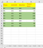
As you can see in the sample, I have a table Phase for my articles to be made in separate machines, and how many peaces done by the same one.

In some cases, the same piece can be done in two separate machines, but in one machine you can make more pieces.

So I would like to highlight the highest number done.

Thank you.

Cycle Time.xlsx
	A	B	C	D
1	Phase	ArticleID	Machine	Peaces done
2	P1	ID1	M1	150
3	P1	ID1	M2	10
4	P2	ID1	M3	200
5	P2	ID2	M3	200
6	P3	ID2	M4	150
7	P3	ID2	M4	50
8	P4	ID1	M5	80
9	P5	ID1	M6	70
Sheet1

 

[James006]

Hi,
For your Conditional Formatting, you can test

=MAXIFS($D$2:$D$9,$A$2:$A$9,A2)=D2

 

[shinigamilight]

with the little explanation you gave, Just select the data from A2 to the last row and input this formula in conditional formatting

=$D2=MAX(IF($A$2:$A$9=$A2,$D$2:$D$9))

 

[Rostuse]

Hi,
For your Conditional Formatting, you can test

=MAXIFS($D$2:$D$9,$A$2:$A$9,A2)=D2

Hello @James006, thank you, but it does not work.

with the little explanation you gave, Just select the data from A2 to the last row and input this formula in conditional formatting

=$D2=MAX(IF($A$2:$A$9=$A2,$D$2:$D$9))

Sorry for the lack of information @shinigamilight

Here is the actual table.

So, as you can see a piece can have various phases, and the same article can be done in two machines, but in one of them are made more pieces per article per phase.

My question is I want to filter let's say the same piece for the same phase and show the value of the machine that has produced more pieces.

Would be even better, to create a new column, and show the result of the bigger value of the article per phase, and the less to be shown as 0 or "FALSE", but also the article that is made in one machine to be shown its current number because not all articles are done by two machines.

EXAMPLE:

TEMPI_CICLO.xlsx
	A	B	C	D	E	F
13	ArticlePhase	ArticleName	MachineName	WorkingTime	Quantity	RESULT
14	20001	ASA24310025	010 QUICK E 1000	19731	190	190
15	20001	ASA24310025	078 STUDER S33	5899	35	0
16	20001	ASA41470167	010 QUICK E 1000	14205	100	100
17	20001	ASA41470229	078 STUDER S33	6054	40	40
18	20001	ASA41470556	010 QUICK E 1000	2439	17	17
19	20001	ASA41470556	078 STUDER S33	976	6	0
Sheet1

Please ignore the Working time column, I need the results in Quantity.

I will appreciate for your help.

Cycle Time.xlsx
	A	B	C	D	E
3	ArticlePhase	ArticleName	MachineName	WorkingTime	Quantity
4	20001	ASA24310025	010 QUICK E 1000	19731	190
5	20001	ASA24310025	078 STUDER S33	5899	35
6	20001	ASA41470167	010 QUICK E 1000	14205	100
7	20001	ASA41470229	078 STUDER S33	6054	40
8	20001	ASA41470556	010 QUICK E 1000	2439	17
9	20001	ASA41470556	078 STUDER S33	976	6
10	20001	ASA51600481	078 STUDER S33	2858	19
11	20001	ASA60670078	078 STUDER S33	1708	20
12	20001	ASAC03500131	078 STUDER S33	3007	10
13	20001	ASAC0350044	078 STUDER S33	16857	120
14	20001	ASAC0350076	078 STUDER S33	5060	40
15	20001	ASAC0350077	078 STUDER S33	7714	41
16	20001	ASAC0350080	010 QUICK E 1000	11817	91
17	20001	ASAC0350080	078 STUDER S33	197886	1557
18	20001	ASAC0350081	010 QUICK E 1000	9869	68
19	20001	ASAC0350081	078 STUDER S33	55103	330
20	20001	ASAC0410001	078 STUDER S33	35882	1127
21	20001	ASAC55K0002	010 QUICK E 1000	9663	54
22	20001	ASAC55K0002	078 STUDER S33	96993	812
23	20001	ASAC55K0013	010 QUICK E 1000	13519	41
24	20001	ASAC55K0013	078 STUDER S33	34949	208
25	20001	ASAC55K0014	078 STUDER S33	10093	37
26	20001	ASAC55P0002	010 QUICK E 1000	76853	1673
27	20001	ASAC55P0002	078 STUDER S33	127479	1306
28	20001	ASANC350362	010 QUICK E 1000	10900	57
29	20002	ASA24310022	078 STUDER S33	3893	39
30	20002	ASA31400140	078 STUDER S33	2322	11
31	20002	ASA31400310	078 STUDER S33	1839	9
32	20002	ASA31400400	078 STUDER S33	19625	155
33	20002	ASA34310050	078 STUDER S33	0	20
34	20002	ASA24310025	010 QUICK E 1000	9812	198
35	20002	ASA24310025	078 STUDER S33	25236	204
36	20002	ASA41470193	078 STUDER S33	6213	24
37	20002	ASA41470200	078 STUDER S33	250	2
38	20002	ASA41470205	078 STUDER S33	14880	129
39	20002	ASA41470556	078 STUDER S33	10424	62
40	20002	ASAC0350047	078 STUDER S33	7205	40
41	20002	ASAC0350080	010 QUICK E 1000	21078	198
42	20002	ASAC0350080	078 STUDER S33	555901	3406
43	20002	ASAC0350081	078 STUDER S33	54572	388
44	20002	ASAC0410001	078 STUDER S33	138649	1092
PVT varianza

 

[shinigamilight]

ctrl shift enter while entering this formula

=IF(COUNTIFS($B$4:$B$44,B4)=1,E4,IF(E4=MAX(IF($B$4:$B$44=B4,$E$4:$E$44)),E4,0))

 

[Rostuse]

ctrl shift enter while entering this formula

=IF(COUNTIFS($B$4:$B$44,B4)=1,E4,IF(E4=MAX(IF($B$4:$B$44=B4,$E$4:$E$44)),E4,0))

Thank you @shinigamilight , but it needs to show the bigger value of the of the same article, and the small one to be 0, in this case both are 0.

In your example E4 and E5.
F4 needs to be 190 and F5 0.

Thank you so much for trying, I really appreciate.

 

[shinigamilight]

Did you even try the formula , first paste it in your workbook then you will realise why is that the case. It was tested on the bigger table not the smaller one.

 

[Rostuse]

Did you even try the formula , first paste it in your workbook then you will realise why is that the case. It was tested on the bigger table not the smaller one.

Yes I did try it, but I got the same result as you have on the screenshot.

The first article for both machines is 0,0.

Thanks

 

[Rostuse]

Bump, anyone will be willing to help?

Thanks.

 

[kevin9999]

Book1
	A	B	C	D	E	F
3	ArticlePhase	ArticleName	MachineName	WorkingTime	Quantity	RESULT
4	20001	ASA24310025	010 QUICK E 1000	19731	190	0
5	20001	ASA24310025	078 STUDER S33	5899	35	0
6	20001	ASA41470167	010 QUICK E 1000	14205	100	100
7	20001	ASA41470229	078 STUDER S33	6054	40	40
8	20001	ASA41470556	010 QUICK E 1000	2439	17	0
9	20001	ASA41470556	078 STUDER S33	976	6	0
10	20001	ASA51600481	078 STUDER S33	2858	19	19
11	20001	ASA60670078	078 STUDER S33	1708	20	20
12	20001	ASAC03500131	078 STUDER S33	3007	10	10
13	20001	ASAC0350044	078 STUDER S33	16857	120	120
14	20001	ASAC0350076	078 STUDER S33	5060	40	40
15	20001	ASAC0350077	078 STUDER S33	7714	41	41
16	20001	ASAC0350080	010 QUICK E 1000	11817	91	0
17	20001	ASAC0350080	078 STUDER S33	197886	1557	0
18	20001	ASAC0350081	010 QUICK E 1000	9869	68	0
19	20001	ASAC0350081	078 STUDER S33	55103	330	0
20	20001	ASAC0410001	078 STUDER S33	35882	1127	1127
21	20001	ASAC55K0002	010 QUICK E 1000	9663	54	0
22	20001	ASAC55K0002	078 STUDER S33	96993	812	812
23	20001	ASAC55K0013	010 QUICK E 1000	13519	41	0
24	20001	ASAC55K0013	078 STUDER S33	34949	208	208
25	20001	ASAC55K0014	078 STUDER S33	10093	37	37
26	20001	ASAC55P0002	010 QUICK E 1000	76853	1673	1673
27	20001	ASAC55P0002	078 STUDER S33	127479	1306	0
28	20001	ASANC350362	010 QUICK E 1000	10900	57	57
29	20002	ASA24310022	078 STUDER S33	3893	39	39
30	20002	ASA31400140	078 STUDER S33	2322	11	11
31	20002	ASA31400310	078 STUDER S33	1839	9	9
32	20002	ASA31400400	078 STUDER S33	19625	155	155
33	20002	ASA34310050	078 STUDER S33	0	20	20
34	20002	ASA24310025	010 QUICK E 1000	9812	198	0
35	20002	ASA24310025	078 STUDER S33	25236	204	204
36	20002	ASA41470193	078 STUDER S33	6213	24	24
37	20002	ASA41470200	078 STUDER S33	250	2	2
38	20002	ASA41470205	078 STUDER S33	14880	129	129
39	20002	ASA41470556	078 STUDER S33	10424	62	62
40	20002	ASAC0350047	078 STUDER S33	7205	40	40
41	20002	ASAC0350080	010 QUICK E 1000	21078	198	0
42	20002	ASAC0350080	078 STUDER S33	555901	3406	3406
43	20002	ASAC0350081	078 STUDER S33	54572	388	388
44	20002	ASAC0410001	078 STUDER S33	138649	1092	0
Sheet1

Cell Formulas
Range	Formula
F4:F44	F4	=IF(AND(COUNTIF($B$4:$B$44,B4)>0,MAXIFS($E$4:$E$44,$B$4:$B$44,A4)=E4),E4,IF(AND(COUNTIF($B$4:$B$44,B4)>0,MAXIFS($E$4:$E$44,$B$4:$B$44,B4)<>E4),0,E4))