Formula/VBA to determine and display stacked chart

[canthony24]

Is it possible to have a formula or VBA to display a dynamic stacked chart? I have the data and the chart already created, just looking to see if this is possible.

The chart shows the number of vendors and sales % for each. If another cell, let's say A1=4, then display only the 4 vendors in the chart and so on. If A1 changes to 7, then display 7 vendors, with a max of up to 10 vendors in the chart.

Ideas?

 

[Jon Peltier]

Yeah, this can be done, and probably doesn't even need VBA. What does your data look like?

 

[canthony24]

So in Cell B7, I have a countif formula to count the number of suppliers that equals up to 80% of sales. That changes whenever the source data is updated. In another section of the worksheet, I have a list of suppliers reading off of a pivot in another worksheet. It's just a reference formula, up to 10 suppliers since that is max number I want to display. Then that list is building the stacked chart.

This is the chart range, which is referencing from a pivot. A simple '=Pivot_DataZ5' etc etc. If B7 = 6, then show only show 6 suppliers, which will then update the chart. Once I get that figured out, I can make the chart range dynamic. But I'm trying to figure out how to make it so whenever B7 changes, the chart data does as well.

So if B7=10, it would look like this:

	Last 52
COCA COLA	51.0%
PEPSICO	18.5%
COCACOLABOTTLERS SALES&SVC	8.3%
CADBURY SCHWEPPES	6.1%
NATIONAL BEVERAGE CORP	5.0%
COTT BEVERAGES INC	2.6%
WHITE ROCK PRODUCTS	1.3%
TIPP ENTERPRISES NOVAMEX	0.8%
POLAR BEVERAGES	0.7%
RED BULL NORTH AMERICA INC	0.5%

<tbody>
</tbody>

If B7=3, it would look like this:

	Last 52
COCA COLA	51.0%
PEPSICO	18.5%
COCACOLABOTTLERS SALES&SVC	8.3%

<tbody>
</tbody>

<tbody>
</tbody>

 

[Jon Peltier]

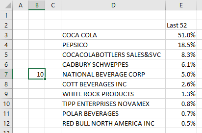
And what is the address of the range containing the 10 or 3 or whatever number of rows? What is the cell address of the cell above "COCA COLA"?

I'll assume the range begins in cell D2, as shown below.

The active cell is D7, which has the number of rows to show.

We'll create a couple dynamic Names that the chart will use.

Go to Formulas tab > Define Name. For Name, enter "xCategories", keep Workbook as Scope, and for Refers To enter this formula and click OK:

=OFFSET(Sheet1!$D$2,1,0,Sheet1!$B$7,1)

This means from our home cell D2, or range is one cell down and zero cells to the right (i.e., D3), and it is B7 rows tall and 1 column wide. So if D7 is 10, it's the range D3:D12. If D7 is 3, it's the range D3:D5.

Return to Formulas tab > Define Name. For Name, enter "yValues", keep Workbook as Scope, and for Refers To enter this formula and click OK:

=OFFSET(xCategories,0,1)

That means from our reference range xCategories, which we've just defined, use the range zero rows down and one column right. So it has the same number of rows as xCategories.

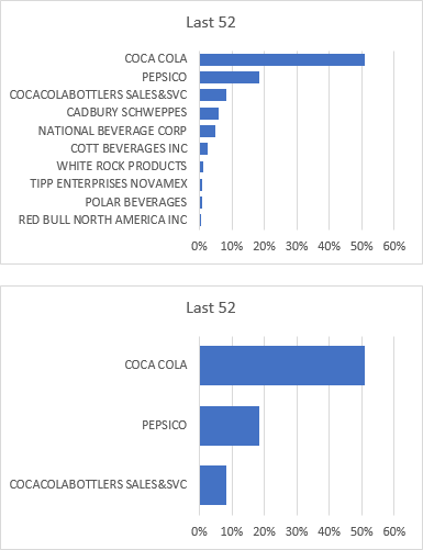
Make your chart with the range D2:E12 (I made a bar chart, first chart below). Click on the series, and notice the formula in the Formula Bar:

=SERIES(Sheet1!$E$2,Sheet1!$D$3:$D$12,Sheet1!$E$3:$E$12,1)

Edit this right in the Formula bar, so it looks like this:

=SERIES(Sheet1!$E$2,Sheet1!xCategories,Sheet1!yValues,1)

Excel will adjust it:

=SERIES(Sheet1!$E$2,'Workbook Name.xlsx'!xCategories,'Workbook Name.xlsx'!yValues,1)

If D7 is 10, it still looks like the top chart. If D7 is 3, it looks like the bottom chart.

I have several similar examples on my web site:

Dynamic Charts
Dynamic Chart Review
Dynamic Chart with Multiple Series
Dynamic Charts in Excel 2016 for Mac

 

[canthony24]

That works perfectly! Thank you so much!

 

[canthony24]

Is there a way to make the list only display the number value selected? So the chart and the list would only show 3, 4 etc?

The chart works perfectly, want to see if the list can do the same.

 

[Jon Peltier]

Your list of companies and percentages link to other cells, right? So still using D2 as my data anchor cell, I would do something like this:

=IF($D$7>=ROW()-ROW($D$2),CellLink,"")

So if D7 is 3, cells D3 through D5 show the linked value and cells D6 and lower show "", so they appear blank.

 

[canthony24]

Where would that formula be entered in?

 

[canthony24]

If I enter it in Cell D2, I get a #Name error.

 

[canthony24]

I figured it out. I was confused on the 'CellLink', but that is the cell I want the data to come from. Thanks for all your help!!