How to return only part of a string from a list?

[FlashDota]

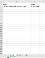
Let's say I have in sheet 1 cell A1: The best scenes from Jursassic Park

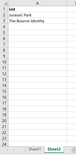
In sheet 2 I have a list like in the picture:
A1: Jursassic Park
A2: The Bourne Identity

I want a formula where if a part of the value in A1 is found in that list, return only that title. See pictures for example

 

[Peter_SSs]

I don't know if it is possible with your data but I included an example in case more than 1 item from Sheet2 is found.

FlashDota.xlsm
	A
1
2	Jurassic Park
3	The Bourne Identity
4	Best Scenes
5
Sheet2

FlashDota.xlsm
	A	B
1
2	The best scenes from Jurassic Park	Jurassic Park, Best Scenes
Sheet1

Cell Formulas
Range	Formula
B2	B2	=LET(r,Sheet2!A$2:A$100,TEXTJOIN(", ",1,FILTER(r,ISNUMBER(SEARCH(r,A2))*(r<>""))))

BTW, I suggest that you investigate XL2BB for providing sample data to make it easier for helpers by not having to manually type out sample data to test with.

 

[MagnarH]

The answer from Petter_SSs is excelent. But I would like add a few points.
Use tabels for both your lists, so it is easier to expand.

Second is add an IFERROR function, in case there NO matches.

My example without the LET-function, but with table ref instead.

=IFERROR(TEXTJOIN(", ",TRUE,FILTER(MyList[List],ISNUMBER(SEARCH(MyList[List];A2))*(MyList[List]<>""))),"Not in list")

 

[Fluff]

There is no reason to use Iferror, which will hid any error, just use the Ifempty argument of filter

=LET(r,Sheet2!A$2:A$100,TEXTJOIN(", ",1,FILTER(r,ISNUMBER(SEARCH(r,A2))*(r<>""),"Not in list")))

 

[MagnarH]

There is no reason to use Iferror, which will hid any error, just use the Ifempty argument of filter

I stand corrected.

Habbits die hard.

 

[FlashDota]

I don't know if it is possible with your data but I included an example in case more than 1 item from Sheet2 is found.

FlashDota.xlsm
	A
1
2	Jurassic Park
3	The Bourne Identity
4	Best Scenes
5
Sheet2

FlashDota.xlsm
	A	B
1
2	The best scenes from Jurassic Park	Jurassic Park, Best Scenes
Sheet1

Cell Formulas
Range	Formula
B2	B2	=LET(r,Sheet2!A$2:A$100,TEXTJOIN(", ",1,FILTER(r,ISNUMBER(SEARCH(r,A2))*(r<>""))))

BTW, I suggest that you investigate XL2BB for providing sample data to make it easier for helpers by not having to manually type out sample data to test with.

Thank you very much, I think this is the solution

 

[Peter_SSs]

You're welcome. Thanks for the follow-up. Might be set to include the "Not in list" per @Fluff's modification or return just "" as below if no matches are found.

=LET(r,Sheet2!A$2:A$100,TEXTJOIN(", ",1,FILTER(r,ISNUMBER(SEARCH(r,A2))*(r<>""),"")))