How to transpose when it matches

[mediumrare]

Hello, and thank you for clicking on this.

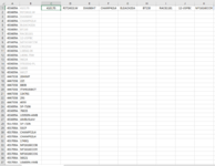
I have a sample spreadsheet for an upcoming inventory project. It has 24,000 lines of products on it. The software we use is able to give me each product that was on an invoice, but I need to put each product on the same row on not on the same column. (Attached is a screenshot. The light grey is where they were and the black is where they should be.

I hope there is a solution for this? I can't tell from my searches whether this is suited for TRANSPOSE, INDEX, MATCH, etc. and how best to apply those to this scenario.


Thanks in advance.

 

[mediumrare]

Added Xl2bb for a test area.

Market Basket Analysis TEST.csv
	A	B	C	D	E	F	G	H	I	J	K
17	444735B	204IMP
18	444735B	225
19	444735B	880B
20	444735B	ITW91930CT
21	444735B	134761
22	444735B	291
23	444735B	4050
24	455699A	SP-7106
25	455699A	76835
26	455699A	US950N-AMB
27	455699A	AMBUSLAV
Market Basket Analysis TEST

 

[Fluff]

Should there be a new row for each distinct value in col A?

 

[mediumrare]

Should there be a new row for each distinct value in col A?

Yes, that would be ideal. Each "invoice number" (A) will not have a duplicate "product number" (B), so there would ideally be a new row for each cell that matches each invoice number.

I hope I'm making sense here!

 

[Fluff]

Ok, how about

+Fluff 1.xlsm
	A	B	C	D	E	F	G	H	I	J	K	L
17	444735B	204IMP		444735B	204IMP	225	880B	ITW91930CT	134761	291	4050
18	444735B	225		455699A	SP-7106	76835	US950N-AMB	AMBUSLAV
19	444735B	880B
20	444735B	ITW91930CT
21	444735B	134761
22	444735B	291
23	444735B	4050
24	455699A	SP-7106
25	455699A	76835
26	455699A	US950N-AMB
27	455699A	AMBUSLAV
28
Main

Cell Formulas
Range	Formula
D17:D18	D17	=UNIQUE(FILTER(A17:A1000,A17:A1000<>""))
E17:K17,E18:H18	E17	=TRANSPOSE(FILTER($B$17:$B$1000,$A$17:$A$1000=D17))
Dynamic array formulas.

 

[mediumrare]

Ok, how about

+Fluff 1.xlsm
	A	B	C	D	E	F	G	H	I	J	K	L
17	444735B	204IMP		444735B	204IMP	225	880B	ITW91930CT	134761	291	4050
18	444735B	225		455699A	SP-7106	76835	US950N-AMB	AMBUSLAV
19	444735B	880B
20	444735B	ITW91930CT
21	444735B	134761
22	444735B	291
23	444735B	4050
24	455699A	SP-7106
25	455699A	76835
26	455699A	US950N-AMB
27	455699A	AMBUSLAV
28
Main

Cell Formulas
Range	Formula
D17:D18	D17	=UNIQUE(FILTER(A17:A1000,A17:A1000<>""))
E17:K17,E18:H18	E17	=TRANSPOSE(FILTER($B$17:$B$1000,$A$17:$A$1000=D17))
Dynamic array formulas.

Thank you, thank you, thank you!

I also think I understand how this formula works too, which is a bonus in and of itself!

 

[Fluff]

You're welcome & thanks for the feedback.