Hi
I'm having some problems and was hoping I might get some help here having come up with nothing from searching the forum
I want to return the text string in a the Cell to the left of the highest value cell in a non-adjacent range from another worksheet to the one where I'm entering the formula
I've tried using the unweildy forumla below
<colgroup><col width="247"></colgroup><tbody>
</tbody>=INDEX((Quality Checks'!B21,'Quality Checks'!B24,'Quality Checks'!B27,'Quality Checks'!B30,'Quality Checks'!B33),MATCH(MAX((Quality Checks'!C21,'Quality Checks'!C24,'Quality Checks'!C27,'Quality Checks'!C30,'Quality Checks'!C33)),(Quality Checks'!C21,'Quality Checks'!C24,'Quality Checks'!C27,'Quality Checks'!C30,'Quality Checks'!C33),0))
and
=INDEX(Quality Checks'!B3,'Quality Checks'!B6,'Quality Checks'!B9,'Quality Checks'!B12,'Quality Checks'!B15,MATCH(MAX(Quality Checks'!C3,'Quality Checks'!C6,'Quality Checks'!C9,'Quality Checks'!C12,'Quality Checks'!C15),Quality Checks'!C3,'Quality Checks'!C6,'Quality Checks'!C9,'Quality Checks'!C12,'Quality Checks'!C15,0))
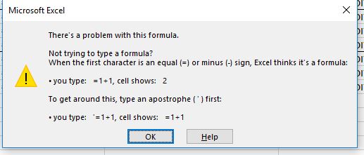
both of which produce this error

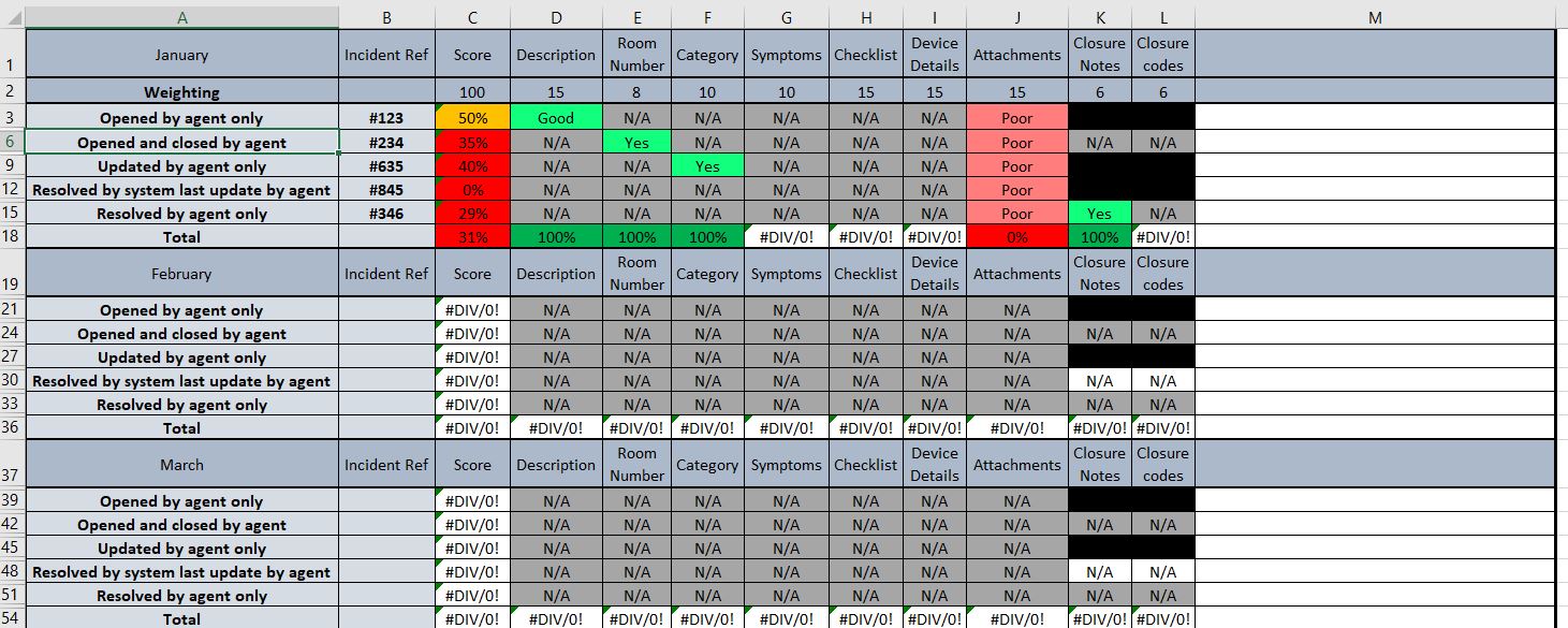
For context this is the sheet that I'm referenceing

As it contain's hidden rows the range is non-adjacent, in the summary sheet I'm trying to build I've got one collumn showing the highest and lowest Score for each month and I want the next colllumn to return the actual Incident Ref.
Any help much appreciated
I'm having some problems and was hoping I might get some help here having come up with nothing from searching the forum
I want to return the text string in a the Cell to the left of the highest value cell in a non-adjacent range from another worksheet to the one where I'm entering the formula
I've tried using the unweildy forumla below
<colgroup><col width="247"></colgroup><tbody>
</tbody>
and
=INDEX(Quality Checks'!B3,'Quality Checks'!B6,'Quality Checks'!B9,'Quality Checks'!B12,'Quality Checks'!B15,MATCH(MAX(Quality Checks'!C3,'Quality Checks'!C6,'Quality Checks'!C9,'Quality Checks'!C12,'Quality Checks'!C15),Quality Checks'!C3,'Quality Checks'!C6,'Quality Checks'!C9,'Quality Checks'!C12,'Quality Checks'!C15,0))
both of which produce this error
For context this is the sheet that I'm referenceing
As it contain's hidden rows the range is non-adjacent, in the summary sheet I'm trying to build I've got one collumn showing the highest and lowest Score for each month and I want the next colllumn to return the actual Incident Ref.
Any help much appreciated