Index and Match with Concatenate

[cpatomba18]

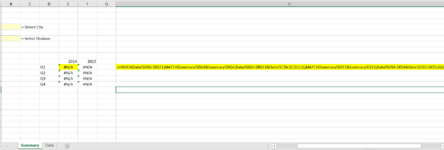
I am trying to retrieve data from a single data tab and output it to a summary tab.

The summary tab has two drop down validations. The 1st is to retrieve the name of the city. The 2nd is to retrieve the name of the division.

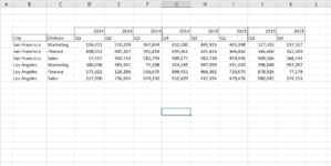
On my data tab, I have two columns - 1st is the city name and 2nd is the division name. I also have two header rows - 1st header row is Year and 2nd header row is Quarter.

My output on the summary tab needs to have the quarter of the calendar year in the column and the year in the row. Right now I am trying a combination of INDEX/MATCH/CONCATENATE as an array function and getting "N/As".

Wondering if this is because my structure in my data set is different from how I want the output?

 

[Toadstool]

Hi CPATomba18,

You can INDEX into a 2D array by specifying the row and column. In your case you need to match 2 items to retrieve both:

1. Row: match City and Division.
2. Column: match Year and Quarter

Here's my test data:

CPATomba18.xlsx
	B	C	D	E	F	G	H	I	J	K
4			2014	2014	2014	2014	2015	2015	2015	2015
5	City	Division	Q1	Q2	Q3	Q4	Q1	Q2	Q3	Q4
6	San Francisco	Marketing	106,782	73,997	55,593	1,556	181,614	64,657	70,910	34,154
7	San Francisco	Finance	138,053	108,899	177,037	186,035	80,181	50,299	33,165	4,031
8	San Francisco	Sales	136,722	68,995	82,085	39,834	70,986	115,065	41,910	189,719
9	Los Angeles	Marketing	84,106	167,423	20,218	171,031	34,736	24,687	95,550	70,036
10	Los Angeles	Finance	98,823	5,108	31,246	1,005	151,941	191,556	12,187	176,756
11	Los Angeles	Sales	92,025	30,270	97,685	70,925	79,865	162,734	9,220	144,662
Datas Tab

Here's my Summary sheet:

CPATomba18.xlsx
	B	C	D	E	F
4	San Francisco	Select City
5
6	Finance	Select Division
7
8
9				2014	2015
10			Q1	138,053	80,181
11			Q2	108,899	50,299
12			Q3	177,037	33,165
13			Q4	186,035	4,031
Summary

Cell Formulas
Range	Formula
E10:F13	E10	=INDEX('Datas Tab'!$D$6:$K$11,MATCH(1,INDEX(('Datas Tab'!$B$6:$B$11=$B$4)*('Datas Tab'!$C$6:$C$11=$B$6),0),0),MATCH(1,INDEX(('Datas Tab'!$D$4:$K$4=E$9)*('Datas Tab'!$D$5:$K$5=$D10),0),0))

Cells with Data Validation
Cell	Allow	Criteria
B4	List	San Francisco,Los Angeles
B6	List	Marketing,Finance,Sales

 

[cpatomba18]

This is fantastic. Thank you very much save me so much headache now trying to figure this out!

 

[Peter_SSs]

Since you have Excel 365, you could also try this.

BTW, I suggest that you investigate XL2BB for providing sample data to make it easier for helpers by not having to manually type out sample data to test with.

cpatomba18.xlsm
	B	C	D	E	F	G	H	I	J	K
4			2014	2014	2014	2014	2015	2015	2015	2015
5			Q1	Q2	Q3	Q4	Q1	Q2	Q3	Q4
6	San Fran	M	475,566	406,937	599,311	574,091	85,159	514,779	452,753	445,999
7	San Fran	F	99,800	221,742	462,932	55,410	439,824	597,162	206,462	266,176
8	San Fran	S	165,446	91,088	461,498	163,797	262,685	160,432	136,749	112,967
9	LA	M	190,999	134,592	288,265	519,849	477,969	384,426	315,470	411,145
10	LA	F	217,752	440,619	97,275	104,233	403,048	501,383	383,331	539,208
11	LA	S	173,460	109,941	226,919	532,522	572,148	64,971	310,430	55,355
Data

cpatomba18.xlsm
	A	B	C	D	E	F
4	LA	City
5
6	F	Division
7
8
9
10					2014	2015
11				Q1	217,752	403,048
12				Q2	440,619	501,383
13				Q3	97,275	383,331
14				Q4	104,233	539,208
Summary

Cell Formulas
Range	Formula
E11:F14	E11	=FILTER(FILTER(Data!$D$6:$K$11,(Data!$B$6:$B$11=$A$4)*(Data!$C$6:$C$11=$A$6)),(Data!$D$4:$K$4=E$10)*(Data!$D$5:$K$5=$D11))

 

[cpatomba18]

Since you have Excel 365, you could also try this.

BTW, I suggest that you investigate XL2BB for providing sample data to make it easier for helpers by not having to manually type out sample data to test with.

cpatomba18.xlsm
	B	C	D	E	F	G	H	I	J	K
4			2014	2014	2014	2014	2015	2015	2015	2015
5			Q1	Q2	Q3	Q4	Q1	Q2	Q3	Q4
6	San Fran	M	475,566	406,937	599,311	574,091	85,159	514,779	452,753	445,999
7	San Fran	F	99,800	221,742	462,932	55,410	439,824	597,162	206,462	266,176
8	San Fran	S	165,446	91,088	461,498	163,797	262,685	160,432	136,749	112,967
9	LA	M	190,999	134,592	288,265	519,849	477,969	384,426	315,470	411,145
10	LA	F	217,752	440,619	97,275	104,233	403,048	501,383	383,331	539,208
11	LA	S	173,460	109,941	226,919	532,522	572,148	64,971	310,430	55,355
Data

cpatomba18.xlsm
	A	B	C	D	E	F
4	LA	City
5
6	F	Division
7
8
9
10					2014	2015
11				Q1	217,752	403,048
12				Q2	440,619	501,383
13				Q3	97,275	383,331
14				Q4	104,233	539,208
Summary

Cell Formulas
Range	Formula
E11:F14	E11	=FILTER(FILTER(Data!$D$6:$K$11,(Data!$B$6:$B$11=$A$4)*(Data!$C$6:$C$11=$A$6)),(Data!$D$4:$K$4=E$10)*(Data!$D$5:$K$5=$D11))

Good to know as well! Thanks!

 

[Peter_SSs]

Good to know as well! Thanks!

You're welcome. Glad to contribute.

 

[Toadstool]

This is fantastic. Thank you very much save me so much headache now trying to figure this out!

You're welcome!

 

[Peter_SSs]

.. another option for all versions too.

cpatomba18.xlsm
	A	B	C	D	E	F
4	LA	City
5
6	F	Division
7
8
9
10					2014	2015
11				Q1	217,752	403,048
12				Q2	440,619	501,383
13				Q3	97,275	383,331
14				Q4	104,233	539,208
Summary (2)

Cell Formulas
Range	Formula
E11:F14	E11	=SUMPRODUCT((Data!$B$6:$B$11=$A$4)*(Data!$C$6:$C$11=$A$6)*(Data!$D$4:$K$4=E$10)*(Data!$D$5:$K$5=$D11),Data!$D$6:$K$11)