INDEX + MATCH; generating more rows

[Martaa]

Hi!

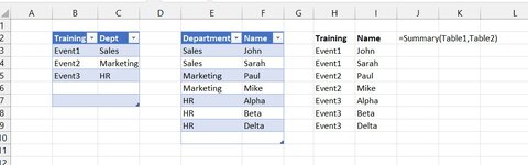
I want to combine 2 tables, and by doing so I want to create a third one which has more rows than the 2 original ones.
I am doing an exercise of organizing trainings in a department.

Here is a picture of what I want to get:

As you can see, the 3rd table is the combination of the 1st and the 2nd.

How can I do that?

Thanks A LOT!!!!

 

[Anthony47]

And which Office version do you use?

 

[Martaa]

And which Office version do you use?

Hi Anthony, I use the 2208 version

 

[Anthony47]

Not clear to me which version is that... so I went for a User Defined Formula, that correspond to the following code:

Function Summary(ByRef TB1 As Range, TB2 As Range) As Variant
Dim OArr(), oaInd As Long, cTrain As String, cDept As String
Dim W1, W2, I As Long, J As Long
'
W1 = TB1.Value
W2 = TB2.Value
'
ReDim OArr(1 To 2, 0 To 1)
For I = 1 To TB1.Rows.Count
    cTrain = W1(I, 1)
    If Len(cTrain) > 0 Then
    cDept = UCase(W1(I, 2))
    For J = 1 To TB2.Rows.Count
        If UCase(W2(J, 1)) = cDept Then
            oaInd = oaInd + 1
            ReDim Preserve OArr(1 To 2, 0 To oaInd)
            OArr(1, oaInd) = cTrain
            OArr(2, oaInd) = W2(J, 2)
        End If
    Next J
    End If
Next I
OArr(1, 0) = "Training"
OArr(2, 0) = "Name"
Summary = Application.WorksheetFunction.Transpose(OArr)
End Function

Copy the code into a standard module of your vba project.
Then return to Excel and you can use the "Summary" function, with the following syntax

Summary(Interval1, Interval2)

Interval1 is the Training /Department table; Interval2 is the Department/Name table

So, having the tables as in the figure, I used H2 the formula

=Summary(Table1,Table2)

The formula returns an array: if your XL version supports dynamic arrays then the output will expand for 2 columns and as many rows are necessary.
Otherwise you have to input the formula on a range of X rows by 2 columns as an array formula (ie: using Contr-Shift-Enter)

Try...

Cartel1
	A	B	C	D	E	F	G	H	I	J	K	L
1
2		Training	Dept		Department	Name		Training	Name	=Summary(Table1,Table2)
3		Event1	Sales		Sales	John		Event1	John
4		Event2	Marketing		Sales	Sarah		Event1	Sarah
5		Event3	HR		Marketing	Paul		Event2	Paul
6					Marketing	Mike		Event2	Mike
7					HR	Alpha		Event3	Alpha
8					HR	Beta		Event3	Beta
9					HR	Delta		Event3	Delta
10
11
Foglio3

Cell Formulas
Range	Formula
H2:I9	H2	=Summary(Table1,Table2)
Dynamic array formulas.

 

[Martaa]

Hi Anthony47,

This was of absolute great help! It works PERFECTLY, and it is exactly what I needed.
I appreciate your time and effort.

Thanks again! :D

 

[Martaa]

Not clear to me which version is that... so I went for a User Defined Formula, that correspond to the following code:

Function Summary(ByRef TB1 As Range, TB2 As Range) As Variant
Dim OArr(), oaInd As Long, cTrain As String, cDept As String
Dim W1, W2, I As Long, J As Long
'
W1 = TB1.Value
W2 = TB2.Value
'
ReDim OArr(1 To 2, 0 To 1)
For I = 1 To TB1.Rows.Count
    cTrain = W1(I, 1)
    If Len(cTrain) > 0 Then
    cDept = UCase(W1(I, 2))
    For J = 1 To TB2.Rows.Count
        If UCase(W2(J, 1)) = cDept Then
            oaInd = oaInd + 1
            ReDim Preserve OArr(1 To 2, 0 To oaInd)
            OArr(1, oaInd) = cTrain
            OArr(2, oaInd) = W2(J, 2)
        End If
    Next J
    End If
Next I
OArr(1, 0) = "Training"
OArr(2, 0) = "Name"
Summary = Application.WorksheetFunction.Transpose(OArr)
End Function

Copy the code into a standard module of your vba project.
Then return to Excel and you can use the "Summary" function, with the following syntax

Summary(Interval1, Interval2)

Interval1 is the Training /Department table; Interval2 is the Department/Name table

So, having the tables as in the figure, I used H2 the formula

=Summary(Table1,Table2)

The formula returns an array: if your XL version supports dynamic arrays then the output will expand for 2 columns and as many rows are necessary.
Otherwise you have to input the formula on a range of X rows by 2 columns as an array formula (ie: using Contr-Shift-Enter)

Try...

Cartel1
	A	B	C	D	E	F	G	H	I	J	K	L
1
2		Training	Dept		Department	Name		Training	Name	=Summary(Table1,Table2)
3		Event1	Sales		Sales	John		Event1	John
4		Event2	Marketing		Sales	Sarah		Event1	Sarah
5		Event3	HR		Marketing	Paul		Event2	Paul
6					Marketing	Mike		Event2	Mike
7					HR	Alpha		Event3	Alpha
8					HR	Beta		Event3	Beta
9					HR	Delta		Event3	Delta
10
11
Foglio3

Cell Formulas
Range	Formula
H2:I9	H2	=Summary(Table1,Table2)
Dynamic array formulas.

Hi Anthony47,

As mentioned in the last comment, your suggestion works perfectly! Thanks A LOT!

I would like to add 2 more features to your code though (2 columns painted in blue in the following picture), and I was wondering if you have a clue on how to do it.

I would like to add a 3rd column to the output, being the department each person is in (see column J in the picture), and a 4th column which is the attendance (see column K).
This column indicates if a person has attended the training they were assigned or not, depending on the attendance list, which is painted in yellow.

Thanks again!

Marta

 

[Anthony47]

In this case the code for the function changes to:

Function SummaryXA(ByRef TB1 As Range, TB2 As Range, ByRef Attend As Range) As Variant
Dim OArr(), oaInd As Long, cTrain As String, cDept As String
Dim W1, W2, I As Long, J As Long
'
W1 = TB1.Value
W2 = TB2.Value
'
ReDim OArr(1 To 4, 0 To 1)
For I = 1 To TB1.Rows.Count
    cTrain = W1(I, 1)
    If Len(cTrain) > 0 Then
    cDept = UCase(W1(I, 2))
    For J = 1 To TB2.Rows.Count
    Debug.Print "J=" & J
        If UCase(W2(J, 1)) = cDept Then
            oaInd = oaInd + 1
            ReDim Preserve OArr(1 To 4, 0 To oaInd)
            OArr(1, oaInd) = cTrain
            OArr(2, oaInd) = W2(J, 2)
            OArr(3, oaInd) = W2(J, 1)
            OArr(4, oaInd) = "No"
            For k = 1 To Attend.Rows.Column
                If Attend.Cells(k, 1) = cTrain And Attend.Cells(k, 2) = W2(J, 2) Then
                    OArr(4, oaInd) = "Yes"
                    Exit For
                End If
            Next k
        End If
    Next J
    End If
Next I
OArr(1, 0) = "Training"
OArr(2, 0) = "Name"
OArr(3, 0) = "Dept"
OArr(4, 0) = "Attended"
SummaryXA = Application.WorksheetFunction.Transpose(OArr)
End Function

The syntax:

 SummaryXA(Interval1, Interval2, Interval3)

So I used, in H1:

=SummaryXA(Table1,Table2,M2:N20)

Please update your profile to specify which Office version you use (eg 2019, 365, 2021,...)

MULTI_C30121.xlsm
	A	B	C	D	E	F	G	H	I	J	K	L	M	N
1													Attendance list
2		Training	Dept		Department	Name		Training	Name	Dept	Attended		Training	Attendance
3		Event1	Sales		Sales	John		Event1	John	Sales	Yes		Event1	John
4		Event2	Marketing		Sales	Sarah		Event1	Sarah	Sales	Yes		Event1	Sarah
5		Event3	HR		Marketing	Paul		Event2	Paul	Marketing	Yes		Event2	Paul
6					Marketing	Mike		Event2	Mike	Marketing	No		Event3	Alpha
7					HR	Alpha		Event3	Alpha	HR	Yes		Event3	Delta
8					HR	Beta		Event3	Beta	HR	No
9					HR	Delta		Event3	Delta	HR	Yes
10
11
12
13
Foglio3

Cell Formulas
Range	Formula
H2:K9	H2	=SummaryXA(Table1,Table2,M2:N20)
Dynamic array formulas.