Index Match Max If - Ecommerce Sales Data

[dtechhh]

Hi there,
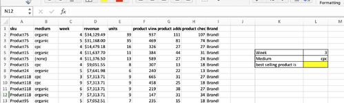
I have an array of e-commerce sales data broken down by week, and source and want to create a formula that tells me the best selling product for each medium each week.

After researching around, I think I need to use a combination of INDEX MATCH & MAX, but haven't found the solution I'm looking for.

I think the solution might be having two input files, Week and Medium, then in a 3rd cell, it returns the highest selling product. (and I just update cells 1 & 2)

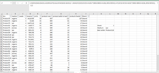
Below is a sample of the data and columns I have to work with.

ecommerce.xlsx
	A	B	C	D	E	F	G	H	I
1	sku	medium	week	revenue	units	product views	product adds to basket	product checkouts	Brand
2	Product75	organic	4	$34,129.49	39	937	111	107	BrandI
3	Product75	organic	5	$31,168.00	35	469	81	74	BrandI
4	Product75	cpc	4	$14,479.18	16	326	27	27	BrandI
5	Product15	organic	4	$11,637.70	11	384	44	31	BrandI
6	Product75	(none)	4	$11,376.50	13	589	27	24	BrandI
7	Product15	cpc	4	$9,051.55	8	307	13	18	BrandI
8	Product24	organic	5	$7,641.98	6	240	22	13	BrandI
9	Product118	cpc	3	$7,313.71	9	665	31	27	BrandI
10	Product118	cpc	9	$7,313.71	9	458	25	18	BrandI
11	Product118	organic	6	$7,313.71	9	219	38	27	BrandI
12	Product118	organic	7	$7,313.71	9	147	31	34	BrandI
13	Product95	organic	5	$7,052.51	7	235	15	18	BrandI
14	Product15	organic	5	$6,583.05	6	209	18	14	BrandI
15	Product118	organic	5	$6,399.50	8	228	21	14	BrandI
16	Product63	organic	4	$6,346.55	7	66	14	13	BrandF
17	Product75	(none)	5	$6,205.36	7	147	16	14	BrandI
18	Product71	organic	10	$5,642.95	5	67	12	13	BrandI
19	Product118	organic	3	$5,485.29	7	211	32	18	BrandI
20	Product75	cpc	5	$5,171.14	6	213	13	11	BrandI
21	Product97	(none)	10	$4,938.17	4	13	2	4	BrandF
22	Product75	cpc	2	$4,701.67	5	66	7	6	BrandI
23	Product75	organic	8	$4,701.67	5	147	16	5	BrandI
24	Product24	organic	8	$4,585.19	4	168	20	11	BrandI
25	Product118	cpc	6	$4,571.07	6	474	26	31	BrandI
26	Product118	cpc	2	$4,571.07	6	464	33	20	BrandI
27	Product118	organic	4	$4,571.07	6	229	27	14	BrandI
28	Product118	organic	8	$4,571.07	6	180	22	14	BrandI
29	Product71	organic	8	$4,232.21	4	145	22	14	BrandI
30	Product63	cpc	2	$4,231.04	5	145	8	8	BrandF
31	Product63	organic	7	$4,231.04	5	95	7	6	BrandF
32	Product12	organic	8	$4,231.04	5	104	11	12	BrandF
33	Product95	organic	7	$4,055.72	4	93	9	8	BrandI
Sheet1

 

[alansidman]

medium	week	Best Seller	BestSales (2).sku
organic	4	34129.49	Product75
organic	5	31168	Product75
cpc	4	14479.18	Product75
(none)	4	11376.5	Product75
cpc	3	7313.71	Product118
cpc	9	7313.71	Product118
organic	6	7313.71	Product118
organic	7	7313.71	Product118
(none)	5	6205.36	Product75
organic	10	5642.95	Product71
organic	3	5485.29	Product118
cpc	5	5171.14	Product75
(none)	10	4938.17	Product97
cpc	2	4701.67	Product75
organic	8	4701.67	Product75
cpc	6	4571.07	Product118

Loaded your table to Power Query Editor and performed Group By

let
    Source = Excel.CurrentWorkbook(){[Name="BestSales"]}[Content],
    #"Grouped Rows" = Table.Group(Source, {"medium", "week"}, {{"Best Seller", each List.Max([#"revenue "]), type number}})
in
    #"Grouped Rows"

Then reloaded original data to PQ Editor

let
    Source = Excel.CurrentWorkbook(){[Name="BestSales"]}[Content]
in
    Source

Then joined the two tables on common fields to get results shown above

let
    Source = Table.NestedJoin(BestSales, {"medium", "week", "Best Seller"}, #"BestSales (2)", {"medium", "week", "revenue "}, "BestSales (2)", JoinKind.LeftOuter),
    #"Expanded BestSales (2)" = Table.ExpandTableColumn(Source, "BestSales (2)", {"sku"}, {"BestSales (2).sku"}),
    #"Changed Type" = Table.TransformColumnTypes(#"Expanded BestSales (2)",{{"Best Seller", Currency.Type}})
in
    #"Changed Type"

 

[dtechhh]

Wow, thanks for the quick reply!

I'm not too familiar with power query and will have to do some further research.


Do you think the solution is solvable with regular excel functions?
I envisage having two input fields, and a 3rd cell returning a value. similar to this screenshot. (green being where the formula is.

 

[shinigamilight]

You never told what criteria you want for the maximum sales, unit or revenue??

Wow, thanks for the quick reply!

I'm not too familiar with power query and will have to do some further research.


Do you think the solution is solvable with regular excel functions?
I envisage having two input fields, and a 3rd cell returning a value. similar to this screenshot. (green being where the formula is.

I chose units for this formula.
Use Ctrl shift enter while entering the formula.

=INDEX($A$2:$A$33,AGGREGATE(14,6,ROW($A$1:$A$32)/--(MAX(IF(($C$2:$C$33=$L$5)*($B$2:$B$33=$L$6),$E$2:$E$33))=IF(($C$2:$C$33=$L$5)*($B$2:$B$33=$L$6),$E$2:$E$33)),1))


I chose revenue for this formula
Use Ctrl shift enter while entering the formula.
=INDEX($A$2:$A$33,AGGREGATE(14,6,ROW($A$1:$A$32)/--(MAX(IF(($C$2:$C$33=$L$5)*($B$2:$B$33=$L$6),$D$2:$D$33))=IF(($C$2:$C$33=$L$5)*($B$2:$B$33=$L$6),$D$2:$D$33)),1))

 

[Fluff]

Another option

Fluff.xlsm
	A	B	C	D	E	F	G	H	I	J	K	L	M	N
1	sku	medium	week	revenue	units	product views	product adds to basket	product checkouts	Brand
2	Product75	organic	4	34129.49	39	937	111	107	BrandI			cpc	2	Product75
3	Product75	organic	5	31168	35	469	81	74	BrandI			cpc	3	Product118
4	Product75	cpc	4	14479.18	16	326	27	27	BrandI			organic	3	Product118
5	Product15	organic	4	11637.7	11	384	44	31	BrandI			(none)	4	Product75
6	Product75	(none)	4	11376.5	13	589	27	24	BrandI			cpc	4	Product75
7	Product15	cpc	4	9051.55	8	307	13	18	BrandI			organic	4	Product75
8	Product24	organic	5	7641.98	6	240	22	13	BrandI			(none)	5	Product75
9	Product118	cpc	3	7313.71	9	665	31	27	BrandI			cpc	5	Product75
10	Product118	cpc	9	7313.71	9	458	25	18	BrandI			organic	5	Product75
11	Product118	organic	6	7313.71	9	219	38	27	BrandI			cpc	6	Product118
12	Product118	organic	7	7313.71	9	147	31	34	BrandI			organic	6	Product118
13	Product95	organic	5	7052.51	7	235	15	18	BrandI			organic	7	Product118
14	Product15	organic	5	6583.05	6	209	18	14	BrandI			organic	8	Product75
15	Product118	organic	5	6399.5	8	228	21	14	BrandI			cpc	9	Product118
16	Product63	organic	4	6346.55	7	66	14	13	BrandF			(none)	10	Product97
17	Product75	(none)	5	6205.36	7	147	16	14	BrandI			organic	10	Product71
18	Product71	organic	10	5642.95	5	67	12	13	BrandI
19	Product118	organic	3	5485.29	7	211	32	18	BrandI
20	Product75	cpc	5	5171.14	6	213	13	11	BrandI
21	Product97	(none)	10	4938.17	4	13	2	4	BrandF
22	Product75	cpc	2	4701.67	5	66	7	6	BrandI
23	Product75	organic	8	4701.67	5	147	16	5	BrandI
24	Product24	organic	8	4585.19	4	168	20	11	BrandI
25	Product118	cpc	6	4571.07	6	474	26	31	BrandI
26	Product118	cpc	2	4571.07	6	464	33	20	BrandI
27	Product118	organic	4	4571.07	6	229	27	14	BrandI
28	Product118	organic	8	4571.07	6	180	22	14	BrandI
29	Product71	organic	8	4232.21	4	145	22	14	BrandI
30	Product63	cpc	2	4231.04	5	145	8	8	BrandF
31	Product63	organic	7	4231.04	5	95	7	6	BrandF
32	Product12	organic	8	4231.04	5	104	11	12	BrandF
33	Product95	organic	7	4055.72	4	93	9	8	BrandI
34
Data

Cell Formulas
Range	Formula
L2:M17	L2	=SORT(UNIQUE(B2:C33),{2,1})
N2:N17	N2	=TAKE(SORT(FILTER($A$2:$D$100,($B$2:$B$100=L2)*($C$2:$C$100=M2)),4,-1),1,1)
Dynamic array formulas.