Match a minimum of 3 and a max of 5 numbers for each row and add the number of cells containing the match displaying in G2 along each row

devincentism

New Member
Joined
Jul 30, 2022
Messages
2
Office Version
  1. 2021
Platform
  1. Windows
I would like this in VBA or Formula. I am using MS 2021 Excel.

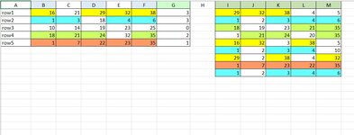
Trying to get Columns B thru F is the numbers assigned to each name in (My Main List) down 5 rows. Rows can be longer but in this example I have it at 5. Columns I thru M I have numbers entered (the entry list) down 10 rows but can be longer. I need see how many matches in each row of of my main list (B2:F2) matches all the cells along each row in my entry list (I2:M2) and Matching at least 3 out of 5 numbers.

Then each match it finds it increments and Displays totals at column G2:G6 and down along each row it matches.

I uploaded an image. In this example this is what I want my totals to be in G2:G6. Any help would be appreciated!
 

Attachments

  • ExcelExample.jpg
    ExcelExample.jpg
    89.4 KB · Views: 9

Excel Facts

What did Pito Salas invent?
Pito Salas, working for Lotus, popularized what would become to be pivot tables. It was released as Lotus Improv in 1989.
Try this in G2:
Excel Formula:
=SUM(IF(MMULT(SIGN(IFERROR(XMATCH($I$2:$M$10,B2:F2),0)),SEQUENCE(COLUMNS($I$2:$M$10),,,0))>=3,1))
 
Upvote 0
Solution
Here is another try at it. But, I do not get your expected results. Can you recheck what your expectations are. I am unsure why you want to read accross the second matrix instead of down, but I have offered two solutions, one down, and one accross:

Mr excel questions 66.xlsm
ABCDEFGHIJKLM
1looking down the column
2ABCDEFGHIJKLM
3row11621293238329323845
4row2131846012346
5row3101419232521819232135
6row418212432351121242035
7row517222335316323385
8123410
9Expected:329238432
10317232235
11012346
122
131
14looking across row
15ABCDEFGHIJKLM
16row11621293238329323845
17row2131846412346
18row3101419232521819232135
19row418212432353121242035
20row517222335016323385
21123410
22Expected:329238432
23317232235
24012346
252
261
devinecentism
Cell Formulas
RangeFormula
G3:G7G3=SUM(--($B3:$F3=INDEX($I$3:$M$11,,ROW(G3)-2)))
G16:G20G16=SUM(--($B3:$F3=TRANSPOSE(INDEX($I$3:$M$11,ROW(G16)-15,))))
 
Upvote 0
Fantastic! That is what I needed. Thankyou
The marked solution has been changed accordingly. In your future questions, please mark the post as the solution that actually answered your question, instead of your feedback message as it will help future readers. No further action is required for this thread.
 
Upvote 0

Forum statistics

Threads
1,215,071
Messages
6,122,963
Members
449,094
Latest member
Anshu121

We've detected that you are using an adblocker.

We have a great community of people providing Excel help here, but the hosting costs are enormous. You can help keep this site running by allowing ads on MrExcel.com.
Allow Ads at MrExcel

Which adblocker are you using?

Disable AdBlock

Follow these easy steps to disable AdBlock

1)Click on the icon in the browser’s toolbar.
2)Click on the icon in the browser’s toolbar.
2)Click on the "Pause on this site" option.
Go back

Disable AdBlock Plus

Follow these easy steps to disable AdBlock Plus

1)Click on the icon in the browser’s toolbar.
2)Click on the toggle to disable it for "mrexcel.com".
Go back

Disable uBlock Origin

Follow these easy steps to disable uBlock Origin

1)Click on the icon in the browser’s toolbar.
2)Click on the "Power" button.
3)Click on the "Refresh" button.
Go back

Disable uBlock

Follow these easy steps to disable uBlock

1)Click on the icon in the browser’s toolbar.
2)Click on the "Power" button.
3)Click on the "Refresh" button.
Go back
Back
Top