Need Help in lookup value with multiple criteria

[bhumit]

HI Team,

Need help in attached sheet for looking up value from table with multiple createria which includes 3 column lookup for 2 input and need result from another column with matched createria.

Please help.
In attached sheet
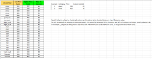
Need D column output by checking G column and H column price checked between B and C column value
For ref, in example 1, category is dress and price is 299 which fall between 292 in B column and 307 in C column, so Output from D column is 49
in example 2, caegory is shirt, price is 425 which fall between 420 in col B and 435 in col C, so output will be 24 from col D

 

[bhumit]

Given table below as i found that i can post directly here.

below is data

cms vertical	Low Price Point	Higher Price Point	New FK Support
dress	292	307	49
dress	370	385	50
dress	540	555	28
dress	600	615	33
dress	690	705	50
jumpsuit	390	405	30
jumpsuit	550	565	30
night_suit	540	555	40
night_suit	590	605	40
shirt	340	355	30
shirt	420	435	24
shirt	690	705	48
skirt	290	305	30
skirt	390	405	30
top	240	255	50
top	290	305	30
top	320	335	35
top	340	355	40
top	400	415	25
top	610	625	35
track_suit	390	405	30
trouser	320	335	45
trouser	390	405	50

Need below result

Example	Category	Price	Output needed
1	dress	299​	49​
2	shirt	425​	24​

Need D column output by checking G column and H column price checked between B and C column value
For ref, in example 1, category is dress and price is 299 which fall between 292 in B column and 307 in C column, so Output from D column is 49
in example 2, caegory is shirt, price is 425 which fall between 420 in col B and 435 in col C, so output will be 24 from col D

 

[Fluff]

Hi & welcome to MrExcel.
How about

Fluff.xlsm
	A	B	C	D	E	F	G	H	I
1	cms vertical	Low Price Point	Higher Price Point	New FK Support		Example	Category	Price	Output needed
2	dress	292	307	49		1	dress	299	49
3	dress	370	385	50		2	shirt	425	24
4	dress	540	555	28
5	dress	600	615	33
6	dress	690	705	50
7	jumpsuit	390	405	30
8	jumpsuit	550	565	30
9	night_suit	540	555	40
10	night_suit	590	605	40
11	shirt	340	355	30
12	shirt	420	435	24
13	shirt	690	705	48
14	skirt	290	305	30
15	skirt	390	405	30
16	top	240	255	50
17	top	290	305	30
18	top	320	335	35
19	top	340	355	40
20	top	400	415	25
21	top	610	625	35
22	track_suit	390	405	30
23	trouser	320	335	45
24	trouser	390	405	50
Home

Cell Formulas
Range	Formula
I2:I3	I2	=FILTER($D$2:$D$100,($A$2:$A$100=G2)*($B$2:$B$100<=H2)*($C$2:$C$100>=H2))

 

[bhumit]

Thanks man, it works

Thank you so much for the help

 

[Fluff]

You're welcome & thanks for the feedback.